Today I brought a somewhat different topic. Have you ever thought it would be great if a compiler could automatically transform loops for optimization or parallelization while using it? Compiler engineers have had the same concerns. One approach that emerged is the polyhedral compiler, which is used by LLVM’s Polly project and MLIR’s affine dialect. Today I’ll introduce this approach.
Basic concepts
Before going into detail, let’s go over some basic concepts. Most of these are easy to encounter with a little linear algebra.
Affine function
An affine function is a function that can be defined as a linear transformation plus a translation. When you apply an affine transformation, points that formed a line move to the same line, and the midpoint of a line segment remains the midpoint after the transformation. In other words, you can think of an affine transformation as allowing a constant term in a linear transformation.
$f(\vec{v})=M_f\vec{v}+\vec{f}_0$
Here, $M$ is a matrix and $\vec{f}_0$ is a constant vector.
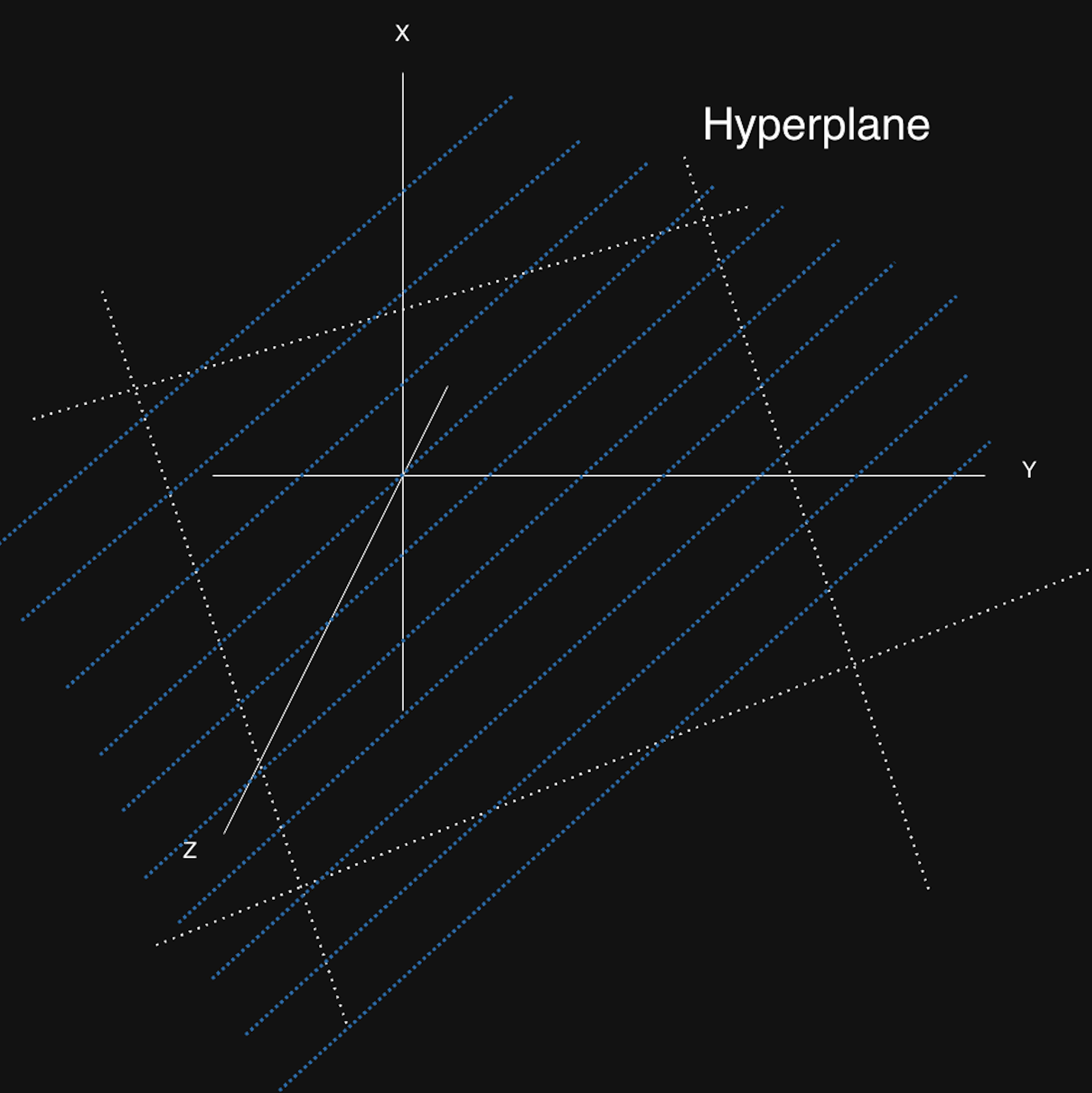
Affine hyperplane
In an n-dimensional space, an affine subspace of dimension n-1 is called an affine hyperplane.
A hyperplane is the set of vectors ($\vec{v}$) that satisfy:
$k = h\vec{v}$ (k is a constant)
So if n is 3, the hyperplane is a 2D plane.
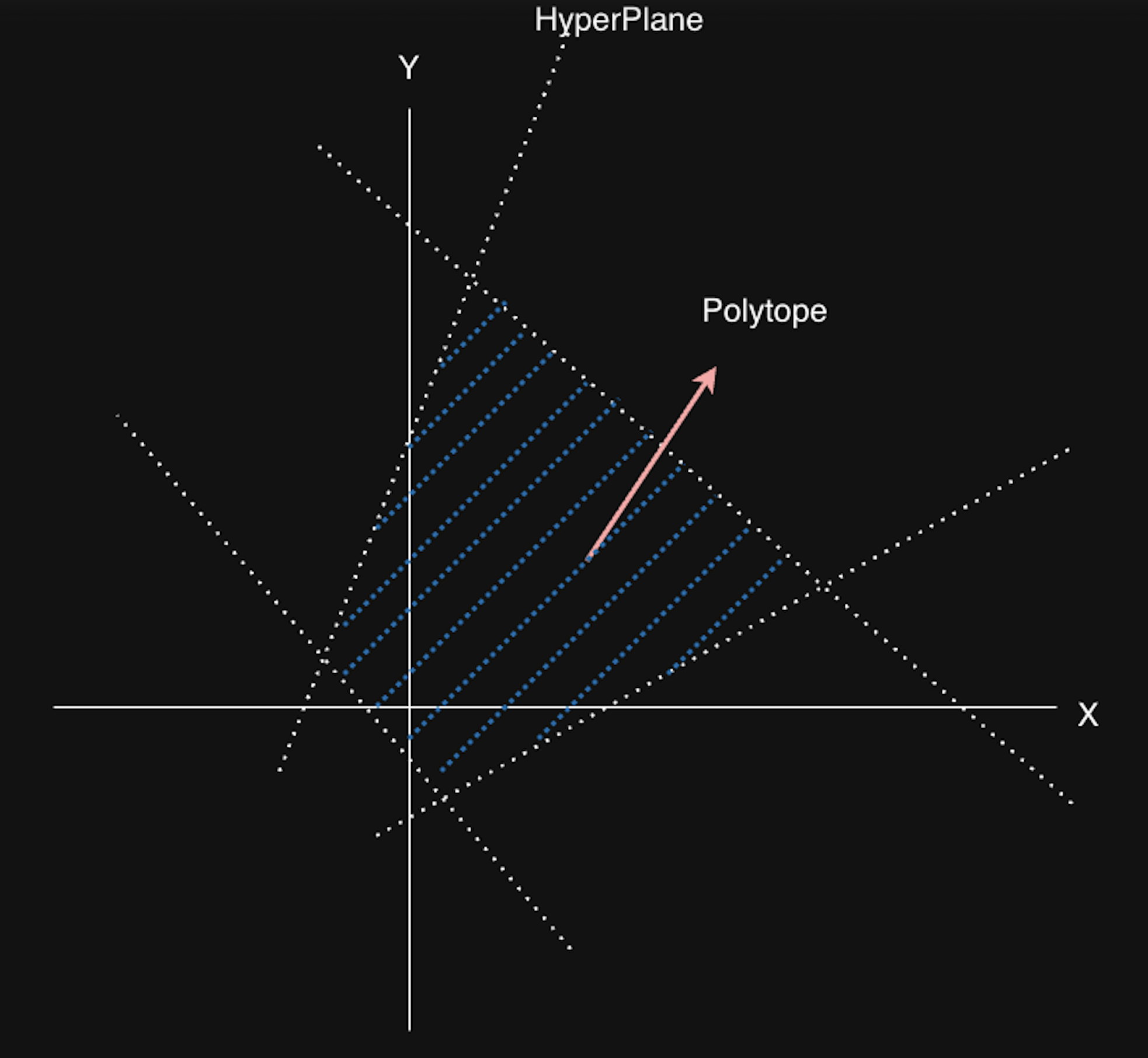
Polyhedron
A polyhedron is the intersection of half-spaces split by a finite number of affine hyperplanes. A bounded polyhedron is called a polytope (meaning it is a closed region).
In the figure below, there are four 1D hyperplanes (since it is a 2D space, the hyperplanes are 1D), and they define a polytope. That is, it is the set of $\vec{x}$ defined by:
${\vec{x} \in \mathbb{R} | A\vec{x} + \vec{b} \ge 0 }$
$A \in \mathbb{R}^{m \times n}, \vec{b} \in \mathbb{R}^m$ (when the polyhedron is bounded by m hyperplanes in n dimensions)
Farkas Lemma
Let the domain $D$ be a polyhedron defined by half-spaces.
Farkas’s lemma states that an affine form (affine function) inside domain D can be expressed as a linear combination of the half-spaces that define D.
In other words, when half-spaces are defined as:
$a_k\vec{x} + b_k ≥ 0, k = 1,p$
it is equivalent that an affine function $\psi(\vec{x})$ is non-negative inside D and that $\psi(\vec{x})$ can be expressed as a linear combination of those non-negative half-spaces.
$\psi(\vec{x}) = \lambda_0 + \sum_{k=1}^{p}\lambda_k(a_k\vec{x} + b_k)\ where \ \lambda_0, \lambda_1, …, \lambda_p \ge 0$
To spell it out, suppose we define an affine function and it lies in domain D. If this function is non-negative, then it can be expressed as a linear combination of the half-spaces that define D, and the converse also holds.
Using this lemma, when transforming a schedule defined by affine functions, we can convert it into a linear combination of half-spaces and solve the problem more easily with ILP.
Interpreting program components
Now that we’ve introduced the basic concepts, let’s see how we can represent a program.
Let’s take a simple example program.
for(int i = 0; i < N; ++i){
  for(int j = 0; j < N; ++j){
    x[i] = x[j]*2 + y[j]; // Statement 1, iteration vector : (i, j)
  }
  for(int k = 0; k < N; ++k){
    y[i] = y[i]*2;        // Statement 2, iteration vector : (i, k)
  }
}
This program consists of three loops and two statements. Each statement has an iteration vector, which is a vector representation of the loop induction variables (iterator variables. i, j and k in the above example.) that affect that statement.
That is, the iteration vector for Statement 1 x[i] = x[j]*2 + y[j] is (i, j),
and the iteration vector for Statement 2 y[i] = y[i]*2 is (i, k).
Schedule vector
A schedule vector indicates when each statement is executed. The schedule vector contains information about the statement’s position and the loops that enclose it.
The schedule vector represents the execution time of a statement, and in polyhedral analysis it is used to check statement conditions or perform transformations.
In the example above, the schedule vector for Statement 1 is (i, 0, j), and for Statement 2 it is (i, 1, k).
The way to set a schedule vector is as follows:
- Describe it from the outermost scope
- If there is a loop, include that loop’s induction variable
- If multiple statements (including loops) exist in a scope, insert a scalar value to separate them (this is called a scalar dimension)
- In the example above, there are two loops inside loop i, so we separated them with a scalar dimension.
- By 1,2,3, the maximum length of a schedule vector is 2m + 1 when there are m nested loops.
<scalar dimension of the outermost scope> + <iteration vector of each loop>*m + <scalar dimension inside each loop> = 2m + 1- Generally, if a scalar dimension is not needed (i.e., there is only one statement in a scope), the scalar dimension is omitted.
Let’s look at another example.
Suppose we have the following code.
for (int i = 0; i < N; ++i) {
    for (int j = 0; j < N; ++j) {
        A[i][j] = A[i][j] + u[i]  * v[j] + u2[i] * v2[j];   // S0
    }
    B[i] = A[i][0]; // S1
}
for (int k = 0; k < N; ++k) {
    for (int l = 0; l < N; ++l) {
        x[k] = x[k] + beta * A[l][k] * y[l];  // S2
    }
}
Then each statement has the following schedule vector:
S0 : $\begin{pmatrix}0&i&0&j\end{pmatrix}$ → the only statement in loop j (index 0) inside loop i (index 0)
S1 : $\begin{pmatrix}0&i&1\end{pmatrix}$ → the first statement (index 1) inside loop i (index 0)
S2 : $\begin{pmatrix}1&k&l\end{pmatrix}$ → the only statement in loop l inside loop k (index 1)
Polyhedral analysis
Now let’s perform polyhedral analysis. First, let’s analyze whether loops can be parallelized.
Parallelism analysis
Consider the following code. Can it be parallelized?
// Q. can loop i and loop j be parallelized?
for(int i = 0; i < N; ++i){
  for(int j = 0; j < N; ++j){
    if(i > j)
      b[i][j] = b[j][i]; // S0
  }
}
What conditions are required to enable parallelization? To parallelize loop i or loop j, there must be no relations between iterations. If each iteration runs independently, that’s fine, but if something written in one iteration must be read in another iteration (or vice versa), you cannot parallelize the loop. So what about the example above?
This code transposes matrix B. It moves the upper-triangular matrix to the lower-triangular matrix. Therefore, there is no relation between loop iterations (no dependency), so it can be parallelized.
Then how can we tell this with polyhedral analysis? We can determine it through a few steps.
- Compute the iteration vector for each statement.
- Represent the domain based on the iteration vector.
- Check whether the domain is empty.
The iteration vector of S0 is (i, j). And S0 has two operations: read and write.
So, viewing S0 from the read and write perspectives:
Read_s0(i, j) = (j, i)
Write_s0(i, j) = (i, j)
And the polyhedron (domain $D_{s0}$) of S0 is defined as:
- i ≥ 0 && i < N
- j ≥ 0 && j < N
- i > j
For a memory dependency to exist, the following must hold:
$$ \exists(\vec{s}, \vec{t}) : \begin{cases} \vec{s} \in D_{s0} \newline \vec{t}\in D_{s0} \newline W(\vec{s}) = R(\vec{t})\end{cases} $$
Here $\vec{s}$ and $\vec{t}$ are different iteration vectors, and each iteration interprets statement S0 in terms of read and write. That is, to parallelize each loop, when we use different iteration vectors, $R(\vec{t})$ (READ_s0(i, j)) must not equal $W(\vec{s})$ (WRITE_s0(i, j))).
Now, let $\vec{s} = (i, j)$ and $\vec{t} = (i’ ,j’)$ and substitute them directly.
Expanding $W(\vec{s}) = R(\vec{t})$ gives $(i’, j’) = (j, i)$. Substituting this into the read condition yields $i’ > j’ \implies j > i$, and the write condition is $i > j$.
But $i > j$ and $j > i$ clearly cannot be satisfied at the same time.
Therefore, the dependence polyhedron is empty, so there is no dependency between iterations, and both loop i and loop j can be parallelized. (Since the domain is empty in the first place, there’s no need to build a schedule vector.)
Let’s look at one more example.
for(int i = 0; i < N; ++i){
  for(int j = 0; j < M; ++j){
    a[i][j] = a[i][j-1]; // S0
  }
}
In this case, how can the code be parallelized?
iteration domain
- i ≥ 0 && i < N
- j ≥ 0 && j < M
iteration vector
$$ \exists(s, t) : \begin{cases} \vec{s} \in D_{s0} \newline \vec{t}\in D_{s0} \newline W(\vec{s}) = R(\vec{t})\end{cases} $$
Let’s build a schedule vector with this. Parallel means there is no dependency between schedules, so for all loops to be parallelizable, we must satisfy the following. (If only some are 0, only the loops corresponding to those dimensions are parallelizable.)
($\phi(\vec{s}), \phi(\vec{t})$ are the schedule vectors for each iteration.)
$$ \phi_{s0}(\vec{t}) - \phi_{s0}(\vec{s}) =\vec{0} $$
If we omit scalar dimensions,
$$ \begin{pmatrix}i \newline j \end{pmatrix} - \begin{pmatrix} i’ = i \newline j’ = j-1 \end{pmatrix} = \begin{pmatrix}0 \newline 1 \end{pmatrix} $$
That is, loop i gives 0 and loop j gives 1, so we can see a dependency exists only in loop j. Therefore, in the example above, only loop i can be parallelized.
We also created an example of analyzing parallelism by constructing schedule vectors in this way.
Polyhedral transformation
Now let’s learn about polyhedral transformation. Polyhedral transformation is the process of changing analyzed code into a more efficient form, and it is executed by libraries like llvm-polly for optimization.
The key is to transform the code in a direction that minimizes cost by defining a cost function while preserving correctness.
For the i-th dimension of the schedule vector of statement $S^k$, we can write part of the schedule vector as follows:
$$ \phi_{S_i^k}(\vec{t})=\begin{pmatrix}c_0^i&c_1^i&\cdots&c_n^i\end{pmatrix}\begin{pmatrix}i_0\newline i_1\newline i_2\newline \cdots\newline i_{n-1}\newline 1\end{pmatrix} $$
$c_0^i …c_n^i$ are the transformation parameters found by polyhedral optimization. $c_n^i$ is used to represent a scalar dimension.
Expressing this for all dimensions:
$$ \tau_s \vec{t}=\begin{pmatrix}\phi_{S_i^0}(\vec{t}) \newline\phi_{S_i^1}(\vec{t}) \newline\vdots \newline\phi_{S_i^{k-1}}(\vec{t})\end{pmatrix}=\begin{pmatrix}c_1^0 & c_2^0 & \cdots & c_n^0 \newline c_1^1 & c_2^1 & \cdots & c_n^1 \newline\vdots & \vdots & \ddots & \vdots \newline c_1^{k-1} & c_2^{k-1} & \cdots & c_n^{k-1}\end{pmatrix}\vec{t}+\begin{pmatrix}c_0^0 \newline c_0^1 \newline \vdots \newline c_0^{k-1}\end{pmatrix} $$
Here, $\vec{t}$ is the iteration vector.
Once we determine the parameters in the transformation matrix, we get a new schedule vector. If we then build the program according to the new schedule vector while keeping the previously defined constraints, the program will look a bit different (the loop structure or statement indices may change), but it will still execute correctly after the transformation. In a new structure, it might become parallelizable or might not require temporary variables.
Transformation parameters are typically found by minimizing a cost function via ILP, but we can also consider other methods such as genetic algorithms, Bayesian optimization, and RL.
Let’s think through this in more detail with an example.
for(i = 0; i < N; ++i){
  for(j = 0; j < N; ++j){
    for(k = 0; k < N; ++k){
      c[i][j] = c[i][j] + a[i][k] * b[k][j]; // S1
    }
  }
}
for(i = 0; i < N; ++i){
  for(j = 0; j < N; ++j){
    for(k = 0; k < N; ++k){
      d[i][j] = d[i][j] + e[i][k]*c[k][j]; // S2
    }
  }
}
Now let’s look at a simple transformation example for this code.
Transformation of Statement S1:
$$ \tau_{s_1}(\vec{i}_{s_1}) = \begin{pmatrix} 0 & 1 & 0 \newline 1 & 0 & 0 \newline 0 & 0 & 0 \newline 0 & 0 & 1\end{pmatrix}\begin{pmatrix}i \newline j \newline k \end{pmatrix} + \begin{pmatrix} 0 \newline 0 \newline 0 \newline 0\end{pmatrix} $$
Therefore, the schedule for each dimension is:
$$ (\phi_{S_1}^1, \phi_{S_1}^2, \phi_{S_1}^3, \phi_{S_1}^4) = (j, i, 0, k) $$
Transformation of Statement S2:
$$ \tau_{s_2}(\vec{i}_{s_2}) = \begin{pmatrix} 0 & 1 & 0 \newline 0 & 0 & 1 \newline 0 & 0 & 0 \newline 1 & 0 & 0\end{pmatrix}\begin{pmatrix}i \newline j \newline k \end{pmatrix} + \begin{pmatrix} 0 \newline 0 \newline 1 \newline 0\end{pmatrix} $$
Therefore, the schedule for each dimension is:
$$ (\phi_{S_2}^1, \phi_{S_2}^2, \phi_{S_2}^3, \phi_{S_2}^4) = (j, k, 1, i) $$
This is the new schedule vector. If we name the loops of the vector in order as t0, t1, t3 and construct new loops, we get the following code:
for(t0 = 0; t0 < N; ++t0){
  for(t1 = 0; t1 < N; ++t1){
    for(t3 = 0; t3 < N; ++t3){
      // i -> t1, j -> t0, k -> t3
      c[t1][t0] = c[t1][t0] + a[t1][t3]*b[t3][t0]; // S1
    }
    for(t3=0; t3 < N; ++t3){
      // i -> t3, j -> t0, k -> t1
      d[t3][t0] = d[t3][t0] + e[t3][t1]*c[t1][t0]; // S2
    }
  }
}
This code behaves the same as the original, but the loop structure is slightly different (the outermost loop has been merged). The fact that it produces the same result is guaranteed because we find the transformation matrix parameters with the assumption that they satisfy the constraints (dependencies, etc.) of the original program.
In the end, the core is to find the transformation matrix $\tau_s$ that satisfies all domain constraints while minimizing the cost function, and usually we do this via ILP. For example, in the above example, we can add constraints that the part reading C in statement S2 must execute after the part writing C in statement S1, and constraints on the loop ranges of i, j, k. We then solve the ILP with these constraints.
A more concrete algorithm for finding the optimal transformation matrix will be explained in a later post.
References
Effective Automatic Parallelization AND Locality Optimization Using The Polyhedral Model (Uday, 2008)