Know Your Enemy, Know Yourself, Supplement: Pallas Programming Model
Know Your Enemy, Know Yourself (知彼知己 百戰不殆)
If you know your enemy and know yourself, you need not fear the result of a hundred battles.
This series aims to deeply understand competitors’ hardware for AI accelerator design.
This article covers Pallas, a programming model that enables writing custom kernels on TPU.
Hello, I’m Donghyeon Choi, an engineer on the HyperAccel ML team.
In part 2, we explored TPU’s hardware architecture and software stack. In this article, we’ll take a deeper look at Pallas, one component of the TPU software stack.
In the latest TPU generation, Ironwood, the Pallas programming model plays a crucial role in performance optimization. Pallas is a tool that allows writing custom kernels on TPU, similar to CUDA or Triton. It enables direct control over hardware details while remaining relatively easy to use in a Python environment.
As mentioned in part 2 regarding the limitations of the XLA compiler, automatic compilers often struggle to optimize cutting-edge algorithms. Pallas is the kernel language Google created to overcome these limitations. When announced alongside Ironwood, it was emphasized with the slogan “Extreme performance: Custom kernels via Pallas.” It plays an important role in maximizing TPU performance.
Therefore, as a supplement to this series, we examine the Pallas programming model before moving on. In this article, we’ll explore what Pallas is, why it’s needed, and how it enhances TPU performance.
Background: TPU Architecture and Why Pallas is Needed
To understand Pallas, we first need to understand how TPU differs from CPUs or GPUs.
Traditional Architecture vs TPU’s Systolic Array
Traditional CPU or GPU architectures repeatedly fetch and store data from SRAM to register files for each operation. In operations like matrix multiplication that repeatedly use the same data, this approach causes massive memory bandwidth waste.
TPU solves this by adopting a structure where once-loaded data flows between compute units and is continuously calculated. This is the Systolic Array structure described in part 2.
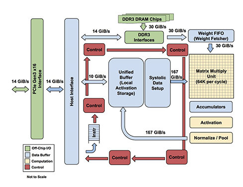
Operations within TPU follow this flow:
- Weight Supply: Weight data stored in DRAM is loaded into Matrix Multiply Unit (MXU) through Weight FIFO.
- Activation Supply: Input data stored in Unified Buffer (UB) is delivered to MXU.
- Matrix Operations: Multiplication and accumulation (Multiply-Accumulate) operations occur simultaneously through the Systolic Array structure inside MXU.
- Post-processing Pipeline: MXU output values pass through Accumulator, Activation Unit (ReLU, etc.), and Normalize/Pool Unit sequentially. These units perform additional operations required by AI models.
- Result Storage: Final output after all operation flows returns to Unified Buffer and is stored.
Key Difference from GPU: Change in Execution Unit
This structural difference creates a very significant difference from a programming model perspective.
- GPU (Single Instruction Multiple Thread, SIMT): Numerous threads perform calculations independently, managed in groups of 32 threads called Warps. It features fine-grained parallel processing focused on individual data.
- TPU (Single Program Multiple Data, SPMD): A single data load completes the entire operation sequence. That is, rather than individual threads, ’the entire program for one tensor (or tile)’ is considered as one minimum execution unit.
Why Pallas? Pallas is a language designed to abstract TPU hardware characteristics (direct Unified Buffer control, MXU scheduling, etc.) while allowing developers to directly optimize this ’tensor-level flow'.
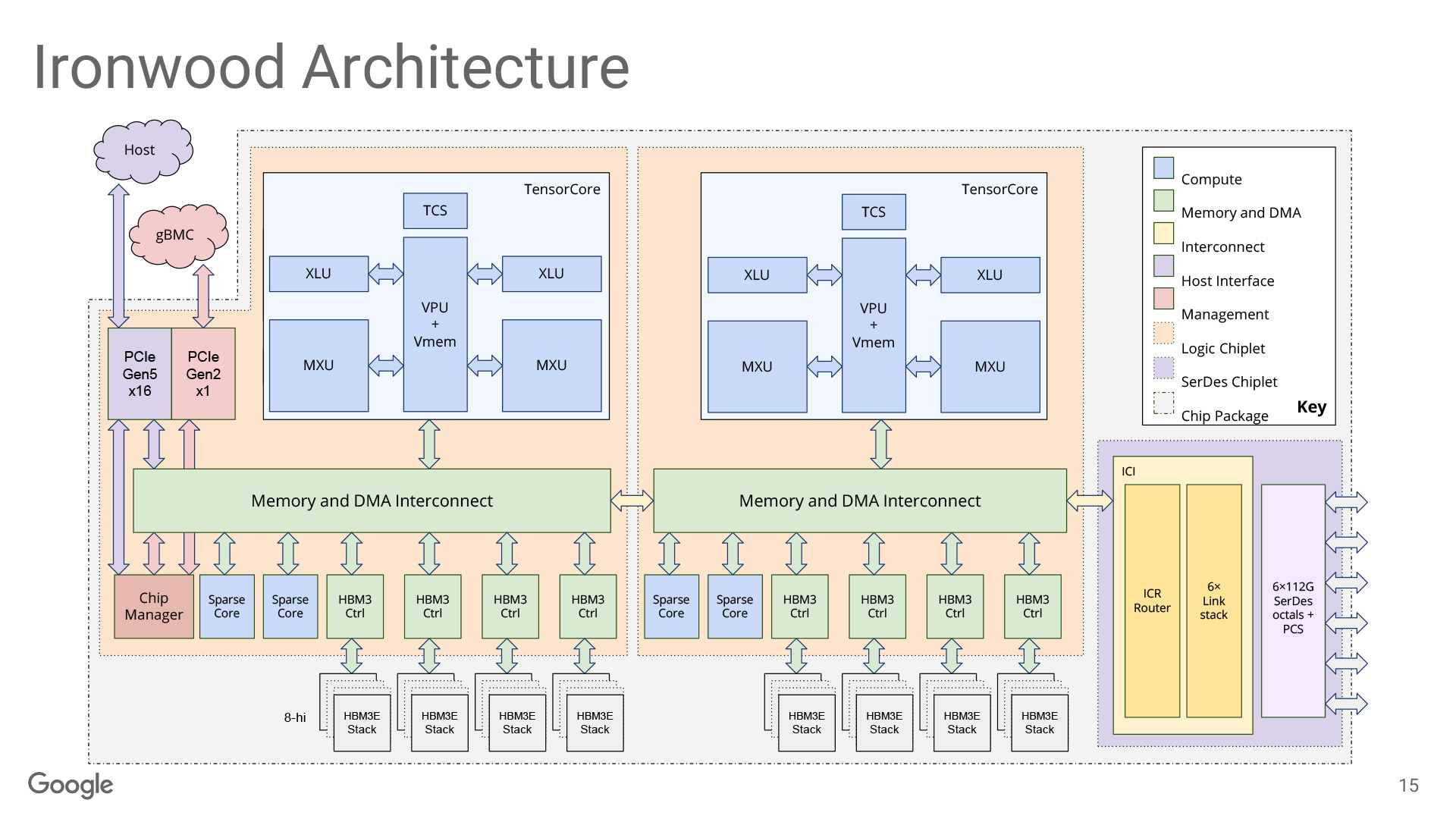
TPU has evolved through generations. It has strengthened vector operation units and developed scale-up technologies for large-scale models. The latest architecture, Ironwood, has become a ‘monster compute unit’ with a massive package adopting chiplet structure and mounting four 256x256 Systolic Arrays (MXU). Despite the dramatic increase in hardware scale, the core design principle remains unchanged: ‘performing as many operations as possible through a single data load’.
Why Pallas is Needed
When we discussed the XLA compiler in part 2, we mentioned that while XLA is a powerful optimization compiler, it has limitations. When new operation algorithms emerge, the compiler struggles to match the performance of manually created custom kernels. This remains true until it’s updated to a version that can optimize them.
For example, cutting-edge algorithms like Flash Attention or MoE (Mixture of Experts) often have complex memory access patterns or high data dependencies. This makes them difficult for automatic compilers to optimize. In such cases, developers need to directly understand the memory hierarchy. They must finely control how to tile data, when to move data between memory levels, and so on.
On GPUs, this problem was solved with CUDA or Triton. CUDA allows direct hardware control but has a high barrier to entry. Triton has a higher level of abstraction, making it relatively easier to use. However, both only work on GPUs.
What about TPU? Google began providing Pallas as an experimental extension of JAX around 2023. Pallas shares a similar philosophy with Triton. It differs significantly in that it supports both GPUs and TPUs.
What is Pallas?
Pallas is a kernel language that enables writing custom kernels within the JAX ecosystem. It works on both GPUs and TPUs. It allows direct control over hardware memory hierarchy, data tiling, and block-level parallelism.
Pallas’s core idea is simple. It allows developers to control operations that are difficult for high-level automated compilers to handle, at a level closer to hardware. Unlike CUDA, it doesn’t go completely low-level. It is abstracted to be relatively easy to use in a Python environment. It finds a balance between the convenience of automatic compilers and the control of manual optimization.
Key Abstractions: Grid, BlockSpec, Ref
Pallas controls hardware through three key abstractions: Grid, BlockSpec, and Ref.
Grid: Parallel Execution Abstraction
Pallas models execution units through a Grid abstraction. Grid has different meanings depending on hardware. It provides a unified interface regardless.
def kernel(o_ref):
    i = pl.program_id(0)  # Current program's ID
    o_ref[i] = i

# Grid size specification: (8,) = 8 parallel programs
result = pl.pallas_call(
    kernel,
    out_shape=jax.ShapeDtypeStruct((8,), jnp.int32),
    grid=(8,),  # 8 parallel instances
)()
In Pallas, Grid is a collection of execution units that divide the entire work. However, how hardware processes this Grid has fundamental differences depending on the architecture.
GPU Grid
In GPU backends (Triton/Mosaic), Grid assumes fully parallel execution by hardware schedulers. Each Grid item is mapped to one Thread Block and executed independently on individual Streaming Multiprocessors (SMs). Since hardware schedules threads non-deterministically, execution order between Grids is not guaranteed. This is an important consideration during development. When designing BlockSpec’s index_map, you must strictly manage race conditions. Different programs must not write to the same High Bandwidth Memory (HBM) location.
TPU Grid
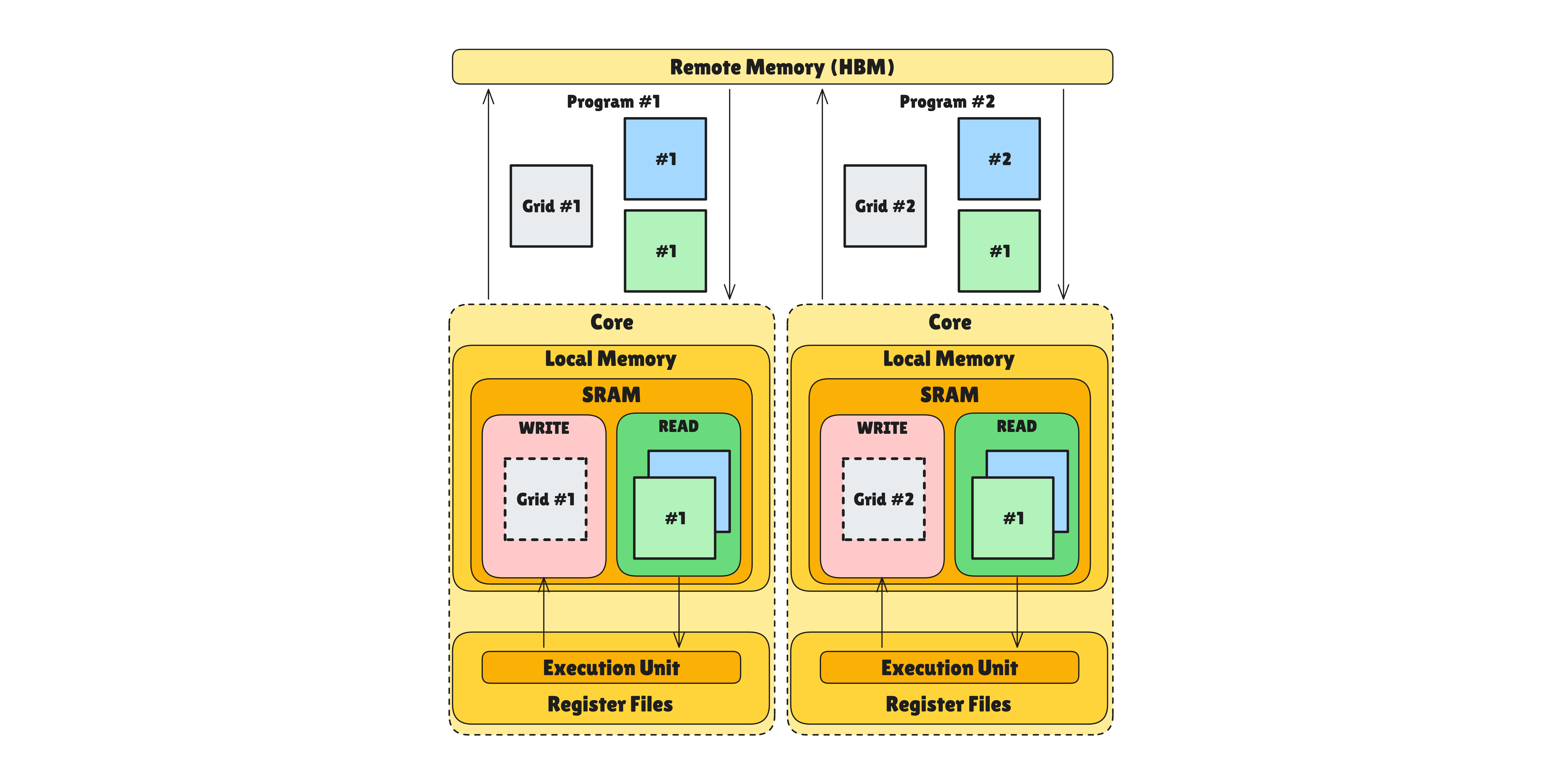
In TPU backends, Grid is a model that combines parallelism between multiple cores and sequential pipelining within a single core.
TPU is a very wide SIMD machine, but can be coded like a single-threaded processor from a software perspective. The Tensor Control System (TCS) provides an intuitive flow that controls entire operations by looping.
When multiple TensorCores exist, there are Parallel dimensions that distribute work and execute physically simultaneously. There are also Sequential dimensions that guarantee serial execution within a single TensorCore. Sequential dimensions are not for slow execution. They are a strategic means to hide memory latency by overlapping current computation with loading of the next data through Semaphores.
BlockSpec: Memory Layout Abstraction
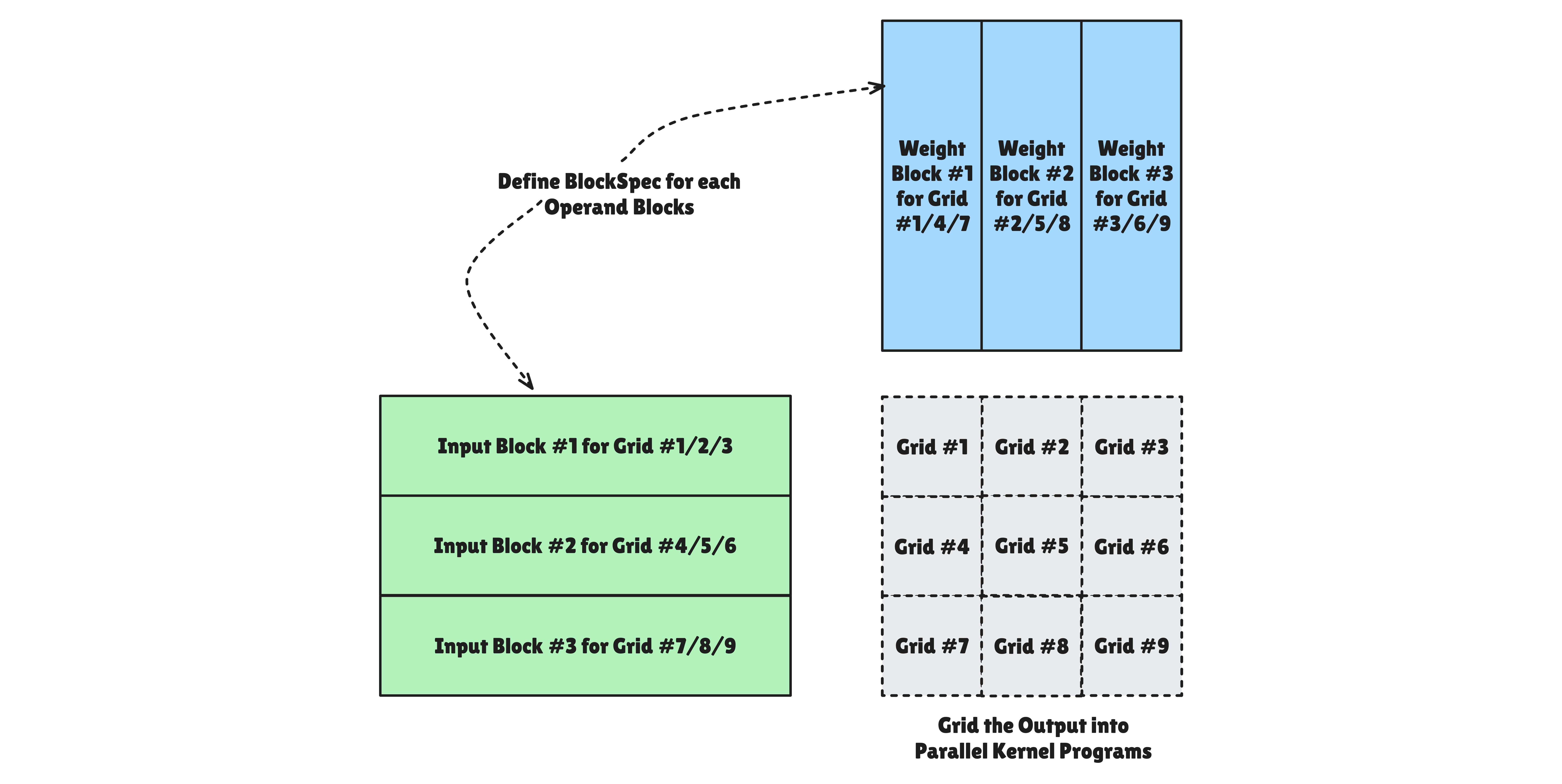
Pallas abstracts the process of dividing massive data into chunks that hardware can digest through BlockSpec. This goes beyond simply cutting data. It defines data transfer protocols between HBM (Remote) and SRAM (Local).
BlockSpec has three components:
block_shape: The size of data that each program instance will place on the Local Memory (SRAM) workbench. Designing this not to exceed hardware SRAM capacity is key to performance optimization.index_mapfunction: Takesgridindices (i, j) as input and returns the block start position on HBM. At compile time, this function is analyzed and converted to hardware Direct Memory Access (DMA) address calculation logic.memory_space: Specifies the physical container where fragmented data will reside. If not specified, it’s allocated to the default space (pl.SRAM) according to backend settings.
Ref: Memory Reference Abstraction
Pallas abstracts complex hardware memory address systems through Ref objects. This goes beyond simple pointers to data and provides a logical view of specific data blocks on SRAM (Local Memory).
Ref’s key features:
- Local Memory Reference:
Refpoints to data on the fastest workbench in hardware—SRAM (TPU’s VMEM/SMEM, GPU’s Shared Memory)—not HBM. The data has already been loaded or will be loaded there. - Dereferencing: When using brackets like
x_ref[...], actual data loading from SRAM → Register File occurs, converting it to aValue. - Hardware Abstraction: Even using the same
Refinterface, it automatically converts depending on the backend. It maps to TPU’s Vector/Scalar memory or GPU’s Shared Memory access. You can also set it directly for clear optimization.
Pallas Hardware Modeling
Pallas provides hardware models for both TPU and GPU. They share the same big picture but differ in details. Let’s first look at the overall structure that’s common to both.
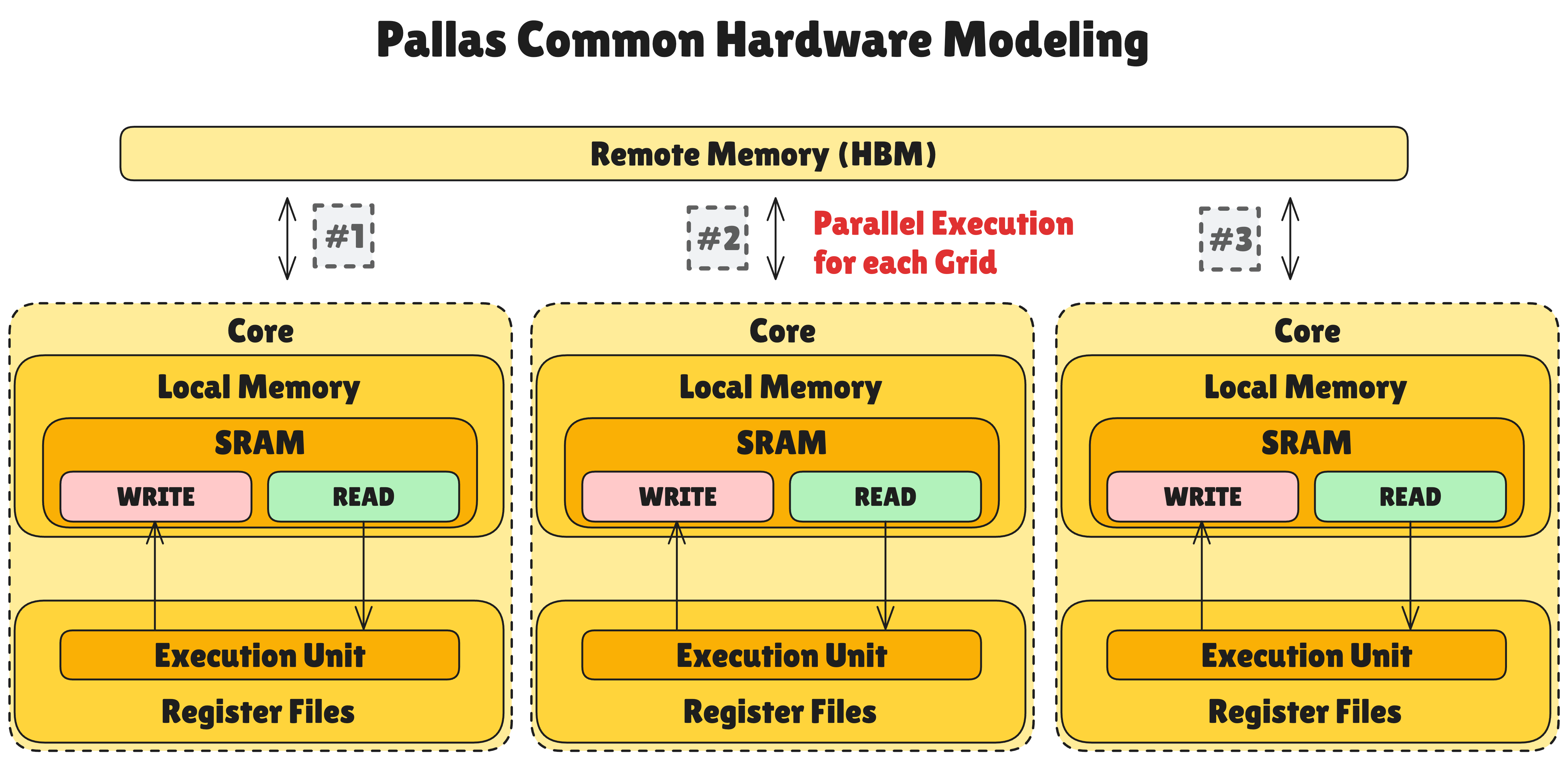
The common hardware model that Pallas abstracts has the following hierarchy:
- Remote Memory (HBM): High Bandwidth Memory—the slowest but highest capacity memory space. Typically specified explicitly through
pltpu.HBMor automatically throughpl.ANY. - Multiple “Core” structure: A collection of independent compute units for parallel grid processing. Each core can perform computations independently.
- Local Memory (SRAM or Cache): Fast memory located inside cores. Much faster than Remote Memory but with limited capacity. Separating READ and WRITE variables is recommended for consistency with HBM data.
- Register Files in Execution Units: The fastest memory that can directly exchange data with compute units. Provides data immediately needed for computation.
Generally, Local Memory takes about 10x the latency of Register File. Remote Memory takes another 10x the latency of Local Memory. However, in TPU v7 Ironwood adopting chiplet structure, one chip contains HBM. For this reason, Remote Memory communication can be 2~5x faster than the previous 10x.
Pallas TPU Hardware Model
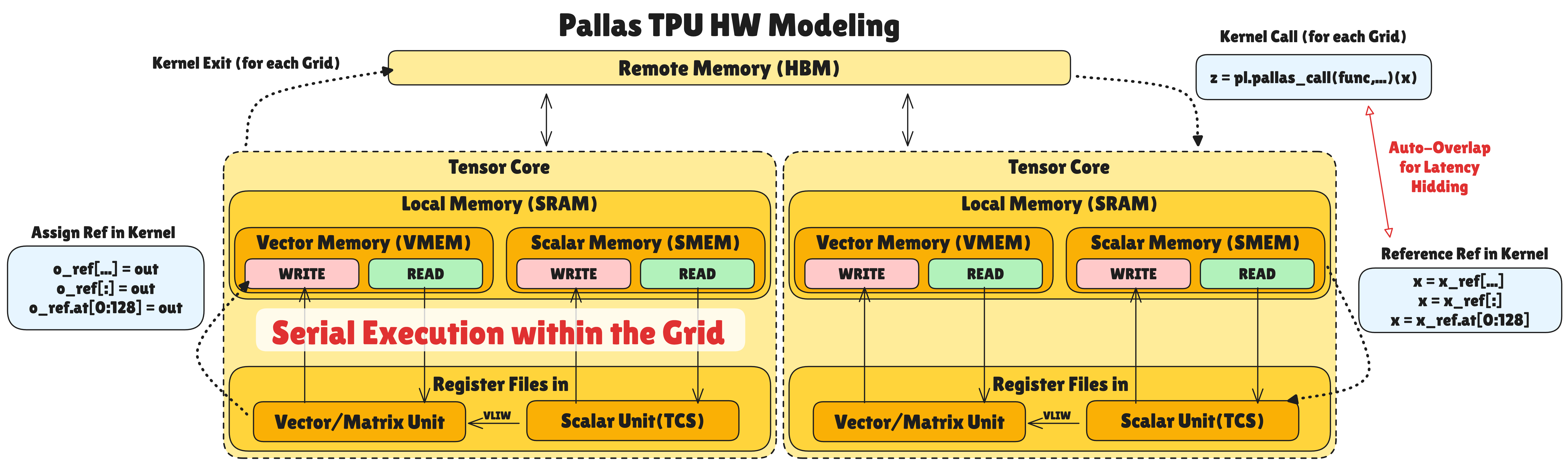
TPU’s hardware model is based on the common model but has TPU-specific structures:
Memory Hierarchy:
Local Memory consists of Vector Memory and Scalar Memory:
- Vector Memory (VMEM): Memory that stores data for Vector and Matrix related operations. Accessible from Vector/Matrix Units (VPU/MXU/XLU) within the same tensor core.
- Scalar Memory (SMEM): Memory that stores data for scalar operations for logic flow (loops, conditions, etc.). Accessible from Scalar Unit (TCS) within the same tensor core. TCS generates high-level commands through which SMEM data can be directly used in vector operations.
Each VMEM and SMEM has separate READ/WRITE areas to ensure data sync with HBM. This is because modifying data read as READ without write-back can cause data inconsistency with HBM.
Data Flow and Pipelining:
When calling a kernel, data is loaded from Remote Memory (HBM) to Local Memory (VMEM/SMEM) according to the specified BlockSpec. Data corresponding to the set Grid number is automatically fetched.
When calling Ref data inside the kernel, data is fetched from Local Memory to Register File for computation. During Local Memory ↔ Register File transfer and computation, data loading from Remote Memory → Local Memory for the next Grid automatically overlaps. This can hide memory latency significantly.
When the kernel writes result data to the configured output Ref, it is written back to Local Memory. When all programs for that grid finish, the output Ref data is written back to Remote Memory.
Pallas GPU Hardware Model
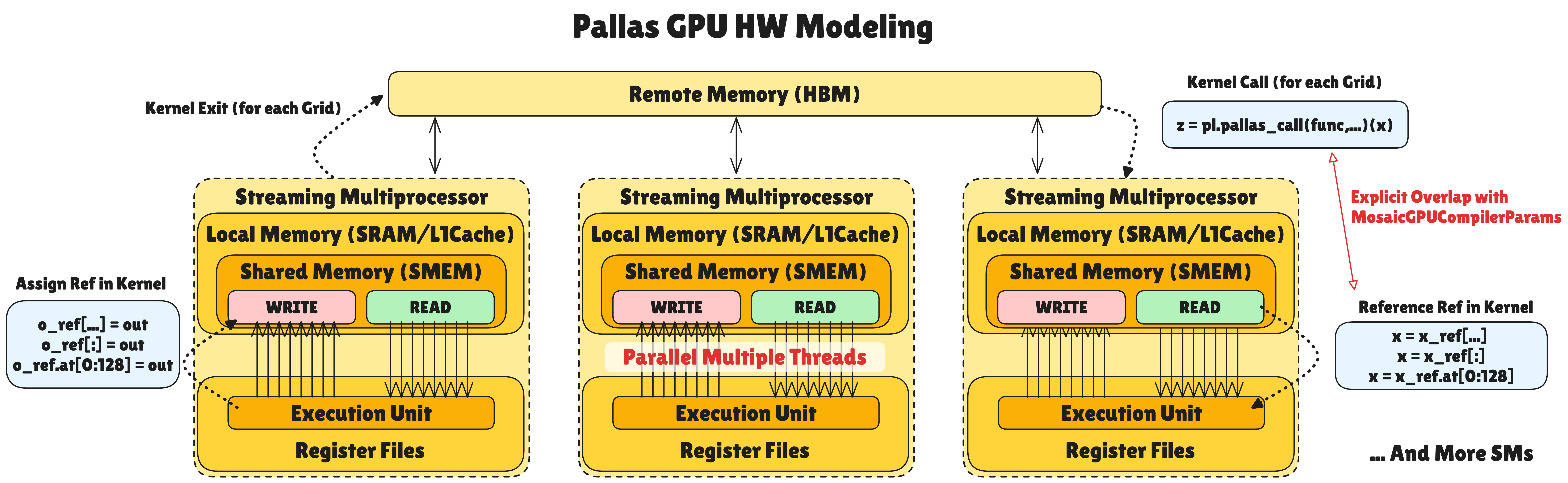
GPU’s hardware model is also based on the common model but has GPU-specific structures:
Memory Hierarchy:
- Local Memory is Shared Memory (SMEM): Each Streaming Multiprocessor (SM) has independent Shared Memory/L1 Cache space. Unlike TPU, it’s a unified workspace without Scalar/Vector distinction. Numerous threads access this space simultaneously for parallel operations.
Data Flow and Pipelining:
Unlike existing methods that rely only on hardware scheduling, Pallas GPU explicitly overlaps HBM (Remote) → SMEM (Local) data loading with TensorCore operations. Through
plgpu.emit_pipeline, etc., compute units process current data while data for the next grid is prefetched asynchronously. This hides memory latency.Ref variables inside kernels are addresses of data chunks on Local Memory (SMEM), not HBM. The data has already been loaded or will be loaded there. Through
memory_space=plgpu.GPUMemorySpace.GMEM, HBM (Remote) space can be explicitly specified. You can control it directly withcopy_gmem_to_smem.
Memory Pipelining and Semaphore
Data movement between HBM (Remote Memory) and VMEM (Local Memory) in TPU architecture causes latency of hundreds of cycles. MXU may perform matrix operations quickly. But if it has to wait for data to arrive, overall performance will be bottlenecked by memory. Pallas solves this with pipelining using hardware-level Semaphores.
Pallas Synchronization Mechanism: Semaphore-based Async Control
In Pallas, DMA and compute units operate independently. Semaphores are used to coordinate their speed difference. The mechanism works as a mutual signaling system:
- Data Load (Producer): When DMA completes loading data from external memory (HBM) to local memory (VMEM/SMEM), it increments (Signals) the semaphore value to indicate that data is ready.
- Compute (Consumer): Compute units check the semaphore value and wait until data is loaded. When the value is satisfied, they immediately start computation.
- Feedback Loop: When computation completes, compute units Signal the semaphore again to notify DMA that the buffer is free, allowing it to load the next data.
Through this Wait-Signal structure, data loading and computation are overlapped for execution, maximizing hardware utilization.
Double Buffering: Key Technique for Hiding Latency
The most basic pipelining technique using semaphores is Double Buffering. Two buffers (Buffer 0, Buffer 1) are allocated within Local Memory, and they operate as follows:
- Initialization: DMA loads the first data into Buffer 0
- Loop Start: While VPU computes Buffer 0, DMA loads the next data into Buffer 1 simultaneously
- Buffer Swap: When both computation and load complete, roles switch—VPU works on Buffer 1, DMA loads into Buffer 0
- Repeat: This process continues until all data is processed
As a result, memory load time is completely hidden behind computation time. Especially effective for compute-bound workloads where computation takes longer than data loading.
Pallas allows explicit control of this synchronization through pltpu.semaphore. It prevents dangerous situations at the hardware level—‘Read-before-ready (reading before data arrives)’ or ‘Write-over-active (overwriting during computation)’. The compiler automatically optimizes Prefetch and Overlap.
Backend Lowering and JAX Integration
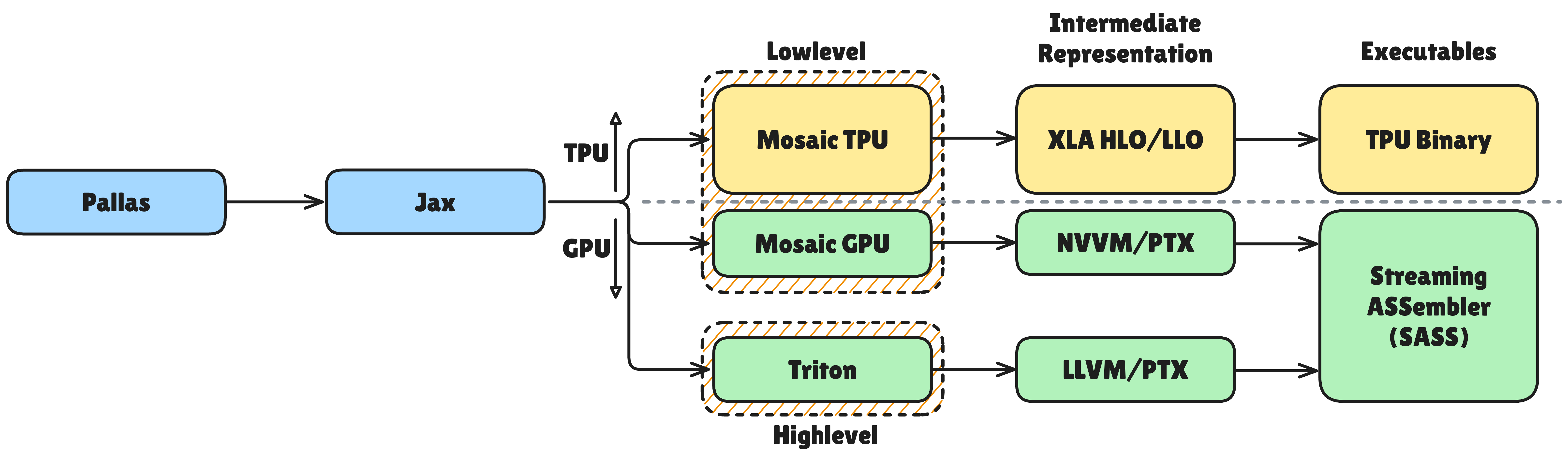
Kernels written in Pallas are eventually converted to hardware code. On GPUs, they are lowered through Triton or Mosaic GPU backends. On TPUs, they are lowered through the Mosaic compiler to MLIR form and finally converted to hardware code. During this process, operator fusion, tiling automation, and overlapping of data transfer and computation are optimized. High-level code written by developers is transformed into hardware-optimized code.
Pallas kernels are also compatible with JAX transforms like jit, vmap, and grad. You can write high-performance kernels while still utilizing automatic differentiation, mapping, and compilation. Pallas is more than a kernel language. It’s a tool fully integrated with the JAX ecosystem.
CUDA vs Pallas: Programming Model Comparison
We compare CUDA from part 1 with Pallas.
Key Comparison
| Category | CUDA | Pallas |
|---|---|---|
| Abstraction | Thread-centric (Thread → Warp → Block → Grid) | Data-centric (Grid + BlockSpec + Ref) |
| Memory Control | Explicit (__shared__, __global__) | Declarative (memory_space, auto mapping) |
| Synchronization | Manual (__syncthreads()) | Automatic (semaphore-based pipelining) |
| Hardware | NVIDIA GPU only | GPU + TPU support |
| Ecosystem | Mature (Nsight, cuBLAS, cuDNN) | Experimental (JAX integration) |
| Language | C/C++ | Python |
Code Comparison: Vector Addition
CUDA - Direct thread ID calculation, boundary check required:
__global__ void vector_add(float *A, float *B, float *C, int N) {
    int idx = blockIdx.x * blockDim.x + threadIdx.x;
    if (idx < N) C[idx] = A[idx] + B[idx];
}
Pallas - Data block-level abstraction:
def vector_add_kernel(a_ref, b_ref, c_ref):
    c_ref[...] = a_ref[...] + b_ref[...]

result = pl.pallas_call(vector_add_kernel, out_shape=..., grid=(N,))(a, b)
This is a conceptual example. For actual execution,
out_shapeandBlockSpecmust be completed.
Selection Guide
| Choose CUDA | Choose Pallas |
|---|---|
| Maximum performance on NVIDIA GPU needed | GPU/TPU portability needed |
| Production stability important | Quick prototyping |
| Leverage existing CUDA codebase | Leverage JAX ecosystem (jit, vmap, grad) |
| Mature debugging/profiling tools needed | Writing TPU custom kernels |
How Pallas is Used on TPU
In the latest TPU generation, Ironwood, Pallas is centered with the slogan “Extreme performance: Custom kernels via Pallas.” In the Ironwood stack, Pallas definitions allow developers to directly describe strategies for memory tiling, data movement, and MXU utilization within Python. The Mosaic compiler lowers this to TPU code.
Through this combination, tiling strategies like input stationary, weight stationary, and output stationary can be efficiently designed. Distributed processing at stride and batch levels can be designed efficiently as well. HBM ↔ on-chip memory data transfer can be overlapped with MXU computation. Designs that minimize scheduling bottlenecks in the entire pipeline are also possible.
Maximum Performance Potential: Memory access patterns and tiling strategies are often difficult for automatic compilers to discover. By adjusting them explicitly, you can create very fast kernels.
Hardware Abstraction Maintained: You still work within the Python language and JAX ecosystem. You can use features like
jitandgradas-is.Multi-Backend Support: Supports both GPUs and TPUs, providing flexibility to run the same kernel definition on multiple hardware platforms.
Considerations
Experimental Stage: Pallas is still in an experimental stage with frequent changes. Breaking changes may occur with version updates. Some features may be incomplete or throw “unimplemented” errors.
Practical Portability: While Pallas has backends for both GPU and TPU platforms, identical code does not run optimally on both systems. Pallas’s portability today is closer to functional compatibility.
Need for Debugging and Optimization Tools: Tools for detailed analysis of MXU utilization, memory bandwidth utilization, etc. are lacking compared to the CUDA ecosystem.
Adoption Barrier: If you have only GPUs without TPUs, using Triton with PyTorch is more practical. Pallas, which is JAX-based and typically requires GCP for TPU access, is difficult to adopt in the general ML stack (PyTorch + AWS or on-premise servers).
Conclusion
In this article, we explored the Pallas programming model that enables writing custom kernels on TPU.
First, we examined how TPU’s Systolic Array structure differs from CPU/GPU. We also looked at how these hardware characteristics affect the programming model. TPU adopts a tensor-centric execution model. It has the structural feature of performing the entire operation sequence through a single data load.
Pallas emerged to address areas difficult for the XLA compiler to automatically optimize. It enables direct control over hardware memory hierarchy and data tiling through the key abstractions of Grid, BlockSpec, and Ref. It provides memory models tailored to TPU and GPU (e.g., TPU’s VMEM/SMEM, GPU’s Shared Memory). It maintains an abstraction level that’s relatively easy to use in a Python environment.
Through comparison with CUDA, we confirmed that Pallas provides a higher level of abstraction while maintaining hardware control. We also saw how Pallas has become a key tool for “Extreme performance” in the Ironwood generation.
Pallas is an important tool that bridges the gap between automated compilers and manual optimization. It enables efficient handling of the complex memory access patterns required by cutting-edge algorithms. As non-standard operation patterns like Flash Attention, MoE, and sparse operations become increasingly important, the role of custom kernel tools like Pallas will only grow.
Reference
- Pallas Documentation
- Pallas TPU Details
- Inside the Ironwood TPU codesigned AI stack
- PyTorch/XLA 2.4 improves Pallas and adds eager mode
- TPU Architecture (qsysarch.com)
- TPU v7 Documentation
P.S. HyperAccel is Hiring!
“Know your enemy, know yourself,” but to win every battle, we need many talented people!
If you’re interested in the technologies we work with, please apply at HyperAccel Career!
HyperAccel has many excellent and brilliant engineers. We’re waiting for your application.