Monads and Category Theory ② Different Computations, the Same Composition

Hello, I am Jaeho Choi from the Compiler team at HyperAccel.

In part 1, we defined composeOption to join two functions whose results might be absent. Option.bind handles the connection between the first function’s result and the next function. The composite is itself a function returning Option, so we can connect another function after it. Even with possible absence, we can keep building larger functions out of smaller ones.

Does this approach work only for Option and missing values? Here we will build composeList, a composition operation for functions that return List.

After finding the common shape of these compositions, we will connect longer sequences of functions. What lets us group consecutive steps differently without changing the result, and account for a sequence with no steps at all? These questions lead us to associativity and the identity laws. We will use Lean 4 to check why composeOption satisfies them, then read the structure we have built through the definition of a category.

1. Connecting functions that return several results

Consider a function that splits a string on spaces into a list of words, and another that turns one word into a list of characters. We want to connect them so that "hi ok" yields ['h', 'i', 'o', 'k']: find the words, find each word’s characters, then concatenate the results in order.

Call the first function $f$ and the second $g$:

f : String → List String   -- split a string into words
g : String → List Char     -- turn a word into characters

Ordinary function composition runs into the same problem we saw in part 1.

g (f sentence)  -- type error: g expects String, not List String

$f$ returns a list of words, List String, while $g$ accepts one word, a String. Merely checking whether a value exists will not connect them. We need to apply $g$ to every word in the list and collect its results.

Let us make the functions concrete in Lean. We define splitWords and give String.toList the name wordChars. These are the $f$ and $g$ above. #eval runs the expression that follows it and displays the result.

def splitWords (s : String) : List String := s.splitOn " "
def wordChars : String → List Char := String.toList

#eval splitWords "hi ok"   -- ["hi", "ok"]
#eval wordChars "hi"       -- ['h', 'i']
#eval wordChars "ok"       -- ['o', 'k']

First, we can connect them by matching on the list directly. An empty list leaves no words to process, so we return []. Otherwise, we obtain the first word’s characters and concatenate them with the characters from the remaining words. This resembles the split between none and some for Option in part 1.

def sentenceCharsByMatch (sentence : String) : List Char :=
  let rec collect (words : List String) : List Char :=
    match words with
    | [] => []
    | word :: rest => wordChars word ++ collect rest
  collect (splitWords sentence)

#eval sentenceCharsByMatch "hi ok" -- ['h', 'i', 'o', 'k']

word :: rest is a list with first word word and remaining words rest. The operator ++ concatenates two lists, and collect rest applies the same rule to the remaining words. For "hi ok", processing the two words eventually reaches collect [], which ends the recursion.

The code computes the result we want. But, as with runOption in part 1, collect mixes an individual computation (wordChars) with a rule for connecting results (++). To use another String → List Char function, such as reverseWordChars, we would have to edit the body of collect.

In part 1, we separated the rule “stop if there is no value; otherwise pass it to the next function” into Option.map and Option.join, then used Option.bind to perform both steps in composeOption. Let us similarly split up the work of collect. First, List.map applies wordChars to every word.

#eval (splitWords "hi ok").map wordChars
-- [['h', 'i'], ['o', 'k']]

The result of map contains all the characters we need, but its type is List (List Char), not the desired List Char. We still have to concatenate the inner lists in order.

Lean calls this operation List.flatten. Applying it to the result of map gives the desired character list.

#eval ((splitWords "hi ok").map wordChars).flatten
-- ['h', 'i', 'o', 'k']

map applied wordChars to each word; flatten concatenated the resulting lists. We have carried out separately the two jobs that were combined in collect.

2. The common shape behind two computations

Now compare Option from part 1 with the List computation above. In both cases, map creates a nested result, although the operation that removes one layer differs.

In part 1, for m : Option B and g : B → Option C, we found (m.map g).join = m.bind g.

For List, Lean’s List.flatMap similarly combines map followed by flatten. For any xs : List B and h : B → List C, we have (xs.map h).flatten = xs.flatMap h.

The two computations remove nesting differently, but both apply the next function and then merge one layer of results. Just as we defined composeOption with Option.bind, let us define composeList with List.flatMap.

def composeList {A B C : Type}
    (f : A → List B) (g : B → List C) : A → List C :=
  fun x => (f x).flatMap g

#eval composeList splitWords wordChars "hi ok"
-- ['h', 'i', 'o', 'k']

To discuss composeOption and composeList together, let $M$ stand for either Option or List. We write the new composition as $\star$ to distinguish it from ordinary function composition $\circ$. The expression $g \star f$ runs $f$ first, then connects $g$: when $M$ is Option, it means composeOption f g; when $M$ is List, it means composeList f g.

Consider $f : A \to M\,B$ and $g : B \to M\,C$ in this notation. Ordinary composition $g \circ f$ would evaluate g (f a) on input a. But f a has type M B, while $g$ expects a B; the expression is ill typed. The new composition $g \star f$ instead passes f a to bind or flatMap along with $g$. Option passes its value to $g$ when one exists, and List passes each element to $g$. Thus $(g \star f)(a) : M\,C$. Two functions that ordinary composition could not connect now form one function of type A → M C.

Let us draw arrows according to this new composition. A function A → M B is an arrow from $A$ to $B$, and B → M C is an arrow from $B$ to $C$. We choose $B$ as the destination of the first arrow because that is the type accepted by the next function. Their composite also has the form A → M C, so it is an arrow from $A$ to $C$.

In our example, splitWords : String → List String returns a list whose elements (String) can be passed to wordChars : String → List Char. In the arrow notation we just chose, we can therefore draw splitWords from String to String, and wordChars from String to Char.

The diagram shows the same relationship for either choice of $M$.

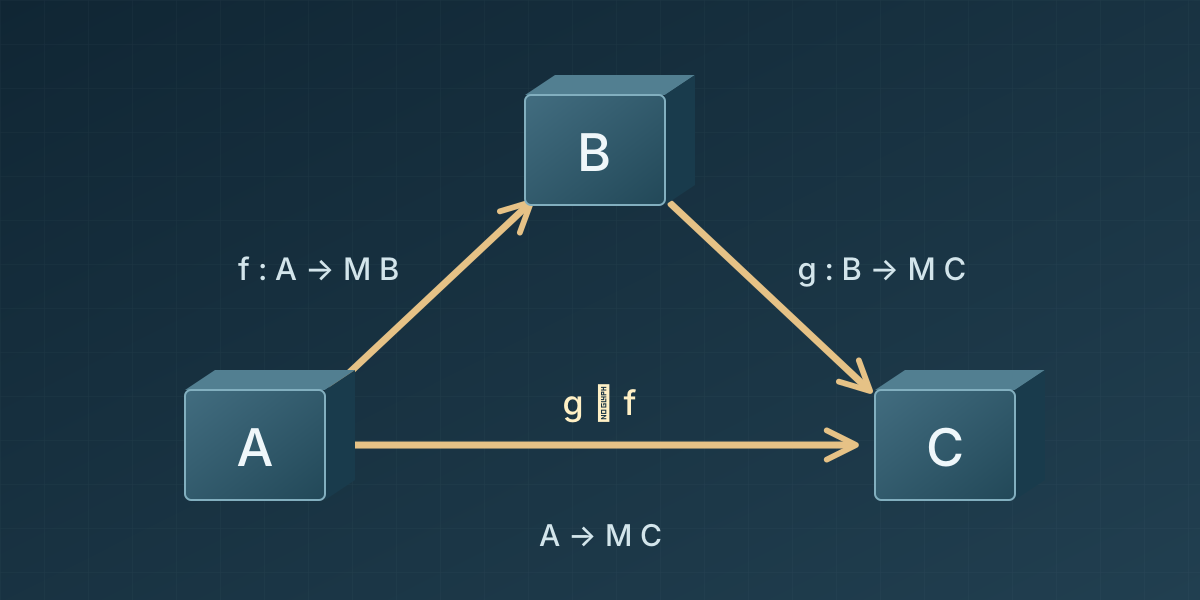
Call a sequence of composable arrows a path. Its length is the number of arrows it contains, so a single arrow is a path of length one. In the diagram, $f$ followed by $g$ is a path of length two; the lower arrow $g \star f$ is its composite. Because this composite has type A → M C, we can append $h : C \to M\,D$ and apply the same operation again.

Having defined $g \star f$ for two arrows, we would like to write the result for three as $h \star g \star f$. But $\star$ combines only two arrows at a time, so we must first choose a pair. Combining $f$ and $g$ gives $h \star (g \star f)$; combining $g$ and $h$ gives $(h \star g) \star f$. If these differ, the unparenthesized expression $h \star g \star f$ does not name a unique composite unless we specify a grouping. Let us ask when the two results coincide.

3. Associativity: does the grouping change the computation?

Consider a path of three arrows, with the following function types:

f : A → M B
g : B → M C
h : C → M D

Joining $f$ and $g$ first gives $g \star f : A \to M\,C$; joining $g$ and $h$ first gives $h \star g : B \to M\,D$. The diagram includes both choices.

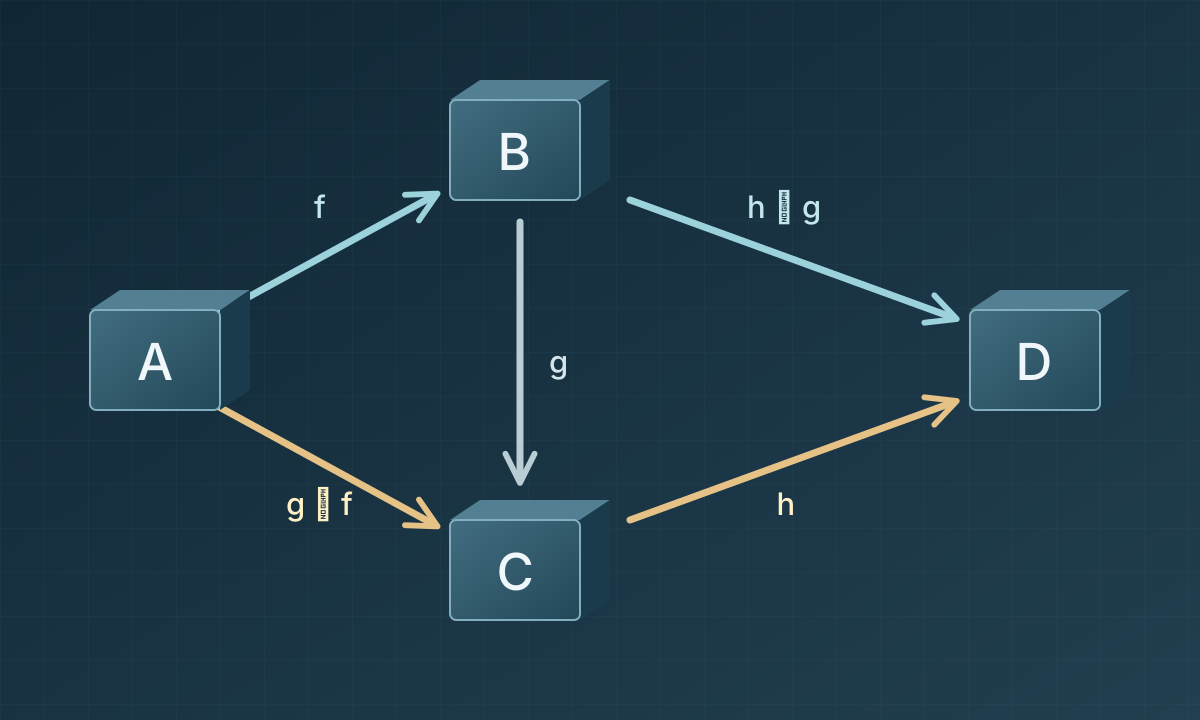
The upper path $A \to B \to D$ groups $g$ and $h$ first, producing $(h \star g) \star f$. The lower path $A \to C \to D$ groups $f$ and $g$ first, producing $h \star (g \star f)$. Both perform $f$, $g$, and $h$ in the same order; they differ only in which portion is composed first.

If the two results agree, we can treat $h \star g \star f$ as one composite arrow without specifying the grouping. This requirement is associativity. When the upper and lower paths give the same arrow, we say the diagram commutes.

h ⋆ (g ⋆ f) = (h ⋆ g) ⋆ f

As a concrete example, append duplicateChar : Char → List Char, which repeats a character, to splitWords and wordChars. If we compose splitWords with wordChars first, we gather all characters and then repeat each one. If we compose wordChars with duplicateChar first, we repeat the characters within each word and then collect the results. Let us compare both computations on "hi ok".

The arguments to composeList are written in execution order. The first expression below groups the first two functions, while the second groups the last two; both still run splitWords, wordChars, and duplicateChar in that order. #guard checks that the following condition is true and reports an error if it is false. Here, == compares the computed result with the expected list.

def duplicateChar (c : Char) : List Char := [c, c]

#guard composeList (composeList splitWords wordChars) duplicateChar "hi ok"
    == ['h', 'h', 'i', 'i', 'o', 'o', 'k', 'k']
#guard composeList splitWords (composeList wordChars duplicateChar) "hi ok"
    == ['h', 'h', 'i', 'i', 'o', 'o', 'k', 'k']

The two expressions agree on "hi ok". This execution alone cannot establish associativity for every choice of functions and input.

If associativity holds, three arrows in the same order give the same result regardless of which pair we compose first. Applying the law repeatedly extends this to four, five, or any finite number of arrows: parentheses do not change the composite. In programming terms, we may move a consecutive group of steps into a helper function and insert that helper back into the original sequence without changing the whole computation.

4. Identity laws: what does “do nothing” mean?

We can now handle a path consisting of f alone, a path that follows f and then g, one that continues through h, and, more generally, a path containing $n$ arrows. With one arrow, we take that arrow itself as the result; with two or more, we compose them in turn. Associativity ensures that a fixed sequence of arrows has the same composite regardless of which part we group first.

Can we take this one step further and handle a path of length zero in the same way? Just as we have assigned a composite arrow to each path, we want to assign an arrow to an empty path that traverses no arrows. A path that starts at $A$ and stays at $A$ must correspond to an arrow whose source and destination are both $A$. Placing an empty path before or after another path adds no computation steps, so composing this arrow must leave the original result unchanged.

For ordinary function composition, id_A : A → A, which returns its input unchanged, plays this role. Composing id_A before a function $p : A \to B$, or id_B after it, leaves $p$ unchanged:

p ∘ id_A = p
id_B ∘ p = p

Our new composition also needs an arrow with this role at each type $A$. But fun x => x has type A → A, not the A → Option A type required of an Option arrow. A candidate for Option is fun x => some x. For List, a candidate is fun x => [x], which turns one input into exactly one result. Returning [] would discard the input before the next computation; returning [x, x] would run that computation twice. Neither preserves it.

We will call the functions that place an ordinary value into these result types pureOption and pureList:

• Candidate identity arrow for Option: pureOption x = some x
• Candidate identity arrow for List: pureList x = [x]

For $f : A \to \text{Option } B$, the candidates on its two sides are $\text{pureOption}_A : A \to \text{Option } A$ and $\text{pureOption}_B : B \to \text{Option } B$. Both equations must hold for our new composition $\star$:

f ⋆ pureOption_A = f    -- wrap first, then run f
pureOption_B ⋆ f = f    -- run f, then wrap its result

In our arrow notation, they look like this:

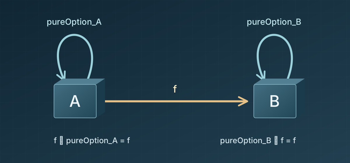
The loops pureOption_A and pureOption_B each start and end at the same object. Traversing the loop at $A$ before $f$, or the loop at $B$ after $f$, must yield the same composite as $f$ itself. These are the two identity laws. When they hold, the loops can serve as the composites of the empty paths at $A$ and $B$.

For List, let us check both directions using wordChars : String → List Char. Wrapping "hi" with pureList yields ["hi"]. Applying flatMap wordChars to that one-element list returns wordChars "hi", or ['h', 'i']. Putting pureList before the computation has left this result unchanged.

In the opposite direction, running wordChars "hi" first yields ['h', 'i']. Wrapping each character with pureList produces [['h'], ['i']]; concatenating these lists gives ['h', 'i'] again. Putting pureList after the computation also preserves the result. The same reasoning applies to empty and longer result lists: each element is wrapped once and then concatenated. Absence and multiplicity are different kinds of computation, but each needs a way to preserve a computation on both sides of composition.

We can check both directions in Lean:

def pureList {A : Type} (x : A) : List A := [x]

#eval (pureList "hi").flatMap wordChars   -- ['h', 'i']
#eval (wordChars "hi").flatMap pureList   -- ['h', 'i']

Like $0$ for addition or $1$ for multiplication, pureOption and pureList provide an element that leaves their respective compositions unchanged.

5. From checking examples to proving the laws

In section 3, we compared two List composites on one input. In section 4, we chose candidate identity arrows for Option and List. Associativity and the identity laws, however, must hold for arbitrary types, functions, and inputs. Let us return to the Option composition from part 1 and prove its laws. An Option result is either none or some b, so we can inspect those two cases.

Instead of running chosen inputs with #eval or #guard, we will state that the two expressions agree for any choice of functions and explain why. Lean checks the claim together with the reasoning. A proof here covers every possible case for an arbitrary input, rather than substituting one particular input.

First, we repeat the definition of composeOption and define its candidate identity arrow pureOption.

-- Option composition and its candidate identity arrow
def composeOption {A B C : Type}
    (f : A → Option B) (g : B → Option C) : A → Option C :=
  fun x => (f x).bind g

def pureOption {A : Type} (x : A) : Option A :=
  some x

5.1. Associativity: the two groupings define the same function

In the notation of section 2, composeOption f g is $g \star f$. We want to prove that grouping f with g gives the same function as grouping g with h. To show that two functions are equal, it suffices to show that they return the same result for every input. This principle is function extensionality.

Take an arbitrary input x and split on the first result f x. If it is none, both groupings return none. If it is some b, both compute g b, stop if its result is absent, and pass its value to h otherwise. The two groupings reduce to the same computation, so they agree for every input.

The code below expresses this argument in a form Lean can check. After theorem, we write the theorem’s name and its arbitrary types and functions; after :, we state the equality to prove. The commands after by construct its proof.

-- Associativity
-- h ⋆ (g ⋆ f) = (h ⋆ g) ⋆ f
theorem composeOption_assoc {A B C D : Type}
    (f : A → Option B) (g : B → Option C) (h : C → Option D) :
    composeOption (composeOption f g) h = composeOption f (composeOption g h) := by
  funext x
  unfold composeOption
  cases f x with
  | none => rfl
  | some b => rfl

funext x uses function extensionality to turn an equality of functions into an equality of their results on an arbitrary input x. unfold composeOption expands the definition of composition, and cases f x splits on the first result. Finally, rfl asks Lean to check that both sides reduce to the same expression using the definitions. Each command corresponds to a step of the argument above.

5.2. Identity laws: inserting an identity leaves a function unchanged

First, connect pureOption after f. When f x is none, it remains none; when it is some b, pureOption b returns some b again. Both cases preserve the original result. In composition notation, this is pureOption ⋆ f = f. The identity arrow appears on the left of the symbol, so this is called the left identity law.

-- Left identity
-- pure ⋆ f = f
theorem composeOption_left_id {A B : Type} (f : A → Option B) :
    composeOption f pureOption = f := by
  funext x
  unfold composeOption pureOption
  cases f x with
  | none => rfl
  | some b => rfl

The proof likewise splits on the two cases of f x; evaluation of the definitions establishes each equality.

Now run pureOption first, then connect f. Because pureOption x is always some x, passing it to Option.bind immediately gives f x. In composition notation, this is f ⋆ pureOption = f. This time the identity arrow appears on the right, giving the right identity law.

-- Right identity
-- f ⋆ pure = f
theorem composeOption_right_id {A B : Type} (f : A → Option B) :
    composeOption pureOption f = f := by
  funext x
  unfold composeOption pureOption
  rfl

The first result is always some x, so this proof needs no case split.

These three theorems prove the laws for every type and function admitted by the declarations. We can also prove the general laws for List. A direct proof uses induction: establish the law for the empty list, then use the result for the rest of a list to establish it after adding one element. Here we focus on the two-case proofs for Option.

You can run the complete example and proofs in the Lean 4 Playground.

6. Different computations, the same rules: categories and Kleisli categories

Option stops when a value is absent; List concatenates multiple results. Yet both compositions we built take a function of the form A → M B as an arrow and produce another arrow of that form. We also examined the associativity and identity laws needed to compose several such arrows.

This resemblance is no accidental coding pattern. The details of the computation differ, but a common structure remains: which arrows we use, how we compose them, and which laws the composition obeys. Mathematics calls these arrows morphisms and calls a structure of objects, morphisms, composition, and identity morphisms satisfying those laws a category. Let us state the definition and see how our proven Option composition fits it.

• Objects: a collection of things from which morphisms start and at which they end.
• Morphisms: for every pair of objects $A,B$, a collection $\mathrm{Hom}_{\mathcal C}(A,B)$ of morphisms from $A$ to $B$. We write a member $f$ as $f : A \to B$; every morphism has a specified source and target.
• Composition: for $f \in \mathrm{Hom}_{\mathcal C}(A,B)$ and $g \in \mathrm{Hom}_{\mathcal C}(B,C)$, a morphism $g \circ f \in \mathrm{Hom}_{\mathcal C}(A,C)$.
• Identity morphisms: for each object $A$, a designated $\mathrm{id}_A \in \mathrm{Hom}_{\mathcal C}(A,A)$. This is the morphism assigned to the empty path at $A$.

The data must satisfy these laws for $f : A \to B$, $g : B \to C$, and $h : C \to D$:

h ∘ (g ∘ f) = (h ∘ g) ∘ f    -- associativity
f ∘ id_A = f                  -- right identity
id_B ∘ f = f                  -- left identity

We say “collection” rather than “set” because the objects of a category cannot always be gathered into a single set. For this series, though, thinking of the objects and morphisms as sets will suffice.

Keeping the objects while changing the morphisms, composition, or identities can give us a different category. We will compare two categories whose objects are types in Lean’s Type. Objects need not be types, and morphisms need not be functions, in an arbitrary category.

6.1. The category $\mathbf{Type}$ of types and ordinary functions

• Objects: types $A,B,C,\dots$ in Lean’s Type.
• Morphisms: $\mathrm{Hom}_{\mathbf{Type}}(A,B)$ consists of functions f : A → B.
• Composition: join f : A → B and g : B → C as g ∘ f : A → C, evaluating g (f a) on input a.
• Identity morphism: id_A : A → A at each type $A$, returning its input unchanged.

These data satisfy the category laws. Whichever pair we compose first among three functions, the result on input a is h (g (f a)). Composing id_A or id_B with $f$ changes no output. We will write this category as $\mathbf{Type}$.

6.2. The Kleisli category for Option

Now keep the same types as objects but use the Option arrows and composition we built. Temporarily call the resulting category $K$.

• Objects: the same types $A,B,C,\dots$.
• Morphisms: $\mathrm{Hom}_K(A,B)$ consists of functions f : A → Option B. We may write them as $A \to_K B$.
• Composition: join f : A → Option B and g : B → Option C as composeOption f g, or $g \star f : A \to \text{Option } C$, evaluating (f a).bind g on input a.
• Identity morphism: pureOption_A : A → Option A at each type $A$, wrapping a as some a.

Calling f : A → Option B a morphism from $A$ to $B$ in this category does not mean changing its return type. f still returns Option B. The diagram shows the difference: the very same function f : A → Option B is a morphism from $A$ to Option B in $\mathbf{Type}$, but a morphism from $A$ to $B$ in the new category.

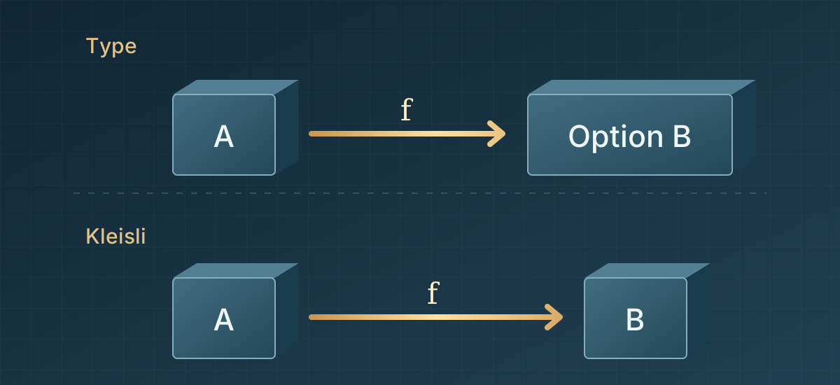
The theorems composeOption_assoc, composeOption_left_id, and composeOption_right_id in section 5 prove the associativity and both identity laws for arbitrary types and functions. Therefore, these data form a category. We call composeOption Kleisli composition and the resulting category the Kleisli category of Option.

Choosing List instead gives a separate Kleisli category with the same types as objects, functions A → List B as morphisms, composeList as composition, and pureList as identity. We do not mix Option and List morphisms within one of these categories. For example, f : A → Option B and g : B → List C cannot be passed directly to either composeOption or composeList. Here we proved the laws for Option in Lean 4 and left the general proof for List aside.

7. The structure we found in composition, and the next question

In part 1, we wanted to connect functions whose results might be absent. Here we extended composition to functions with multiple results and established why regrouping steps can preserve a longer computation. Starting with code that assembles individual functions, we can now describe the mathematical structure supporting that assembly as a category.

In part 3, we will return to $\mathbf{Type}$, whose morphisms are ordinary functions A → B. The category definition above says nothing about a type’s fields or how many values it contains. Yet in programming, we make types that hold two values together, as in a struct, or one of several alternatives, as in an enum. Can we describe these types by the relationships among functions entering and leaving them, rather than by their internal representation?

We will start with functions into the two fields of a struct and functions that handle each case of an enum. Given such functions, we will ask when there is exactly one compatible morphism. A condition that describes an object by the existence and uniqueness of a morphism is called a universal property. Types with the same universal property are isomorphic: inverse functions connect them, even if their internal implementations differ.