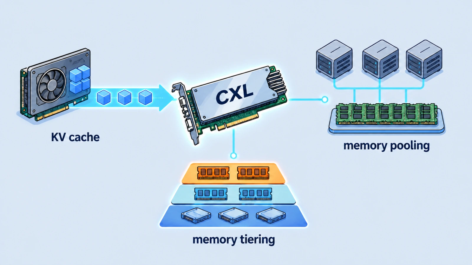
This is Part 5 of the Memory in the AI Era series. Part 1, Part 2, and Part 3 covered High Bandwidth Flash (HBF), which fills a gap in the memory hierarchy next to the GPU. Part 4 shifted to the system level and examined what Compute Express Link (CXL) is. This fifth and final part looks at how CXL is used in real workloads.
Introduction
Hello, I’m Jaewon Lim, an RTL verification engineer at HyperAccel.
In Part 4, we broke down the CXL interface: the gap between DDR and PCIe, the three sub-protocols (CXL.io / CXL.cache / CXL.mem), Type 1/2/3 devices, and the CMM product families from the three major memory vendors.
But I left the most practical question for this installment.
How is CXL used in real LLM serving, and which workloads suit it?
Once we understand the shape of a tool, the next step is to find where it actually fits.
Our starting point is the pair of fundamental properties of CXL discussed in Part 4.
- Benefit: It can extend a large, coherent memory space beyond local memory and distribute capacity among multiple hosts.
- Cost: It is 2-3 times slower than directly attached DDR memory, with latency around 170-300 ns. This is the latency tax.
These properties are two sides of the same coin. The question “Where does CXL fit?” therefore becomes: “Which workloads need capacity and pooling badly enough to absorb this latency tax?”
We will answer that question through three use cases: 1) KV cache offload, 2) VM consolidation through memory pooling, and 3) hot/warm/cold tiering.
This post is based on my personal study and experience. If you find any errors, please let me know in the comments.
Use Case 1 — KV Cache: Memory Forced Out of the GPU
The first role CXL is targeting in LLM serving is as a home for KV cache.
Why KV Cache Becomes a Problem
During LLM inference, the model stores and reuses the Key and Value vectors of all previously generated tokens. This Key-Value cache (KV cache) grows linearly with sequence length and the number of concurrent users.
Its total size can be calculated as follows.
$$\text{KV cache size} = 2 \times B \times S \times L \times H_{kv} \times D_h \times P$$
Here, $B$ is the batch size, $S$ is the sequence length, and $L$ is the number of layers. $H_{kv}$ is the number of KV heads, $D_h$ is the head dimension, and $P$ is the number of bytes per element. The leading 2 accounts for both Key and Value.
For example, serving Llama 3.1 405B with FP8 weights and an FP16 KV cache requires about 516 KB per token. A single user with 100,000 tokens consumes roughly 48 GB. Serving 128 such requests concurrently pushes the KV cache alone to about 6 TB. We covered the calculation in more detail in our earlier NVIDIA ICMS post.
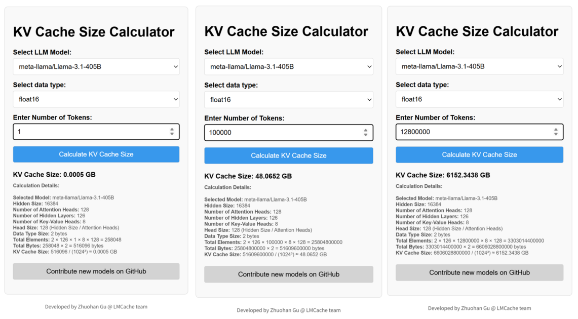
KV cache size calculation for Llama 3.1 405B. Source: LMCache KV Cache Size Calculator
The problem is that this KV cache occupies GPU HBM, the most expensive memory in the system. HBM capacity is limited, and every byte consumed by KV cache reduces the number of requests the GPU can process concurrently.
Limits of Existing Approaches
The industry already moves KV cache out of the GPU. A common approach is to offload it to host DRAM or NVMe SSD and bring it back when needed.
However, GPU HBM, host DRAM, and SSD occupy separate allocation domains. The serving runtime must explicitly track each KV block and manage its movement.
- Host DRAM requires DMA and staging when exchanging data with the GPU.
- NVMe SSD adds block I/O and substantially higher latency.
In either case, software must decide when to move the required KV block back into HBM.
What Changes with CXL?
CXL Type 3 memory enters the host’s physical address space. The CPU can access it through ordinary loads and stores without block I/O. This provides three benefits.
- Capacity: A KV cache space much larger than HBM can be attached to the host address space.
- Access model: The CPU can treat CXL memory as byte-addressable memory.
- Position in the hierarchy: It is a DRAM tier closer than SSD and does not require block I/O.
A public example is SK hynix’s TraCT. TraCT attaches CXL shared memory to NVIDIA Dynamo-vLLM and uses it both as a KV transfer space between prefill and decode GPUs and as a rack-level prefix cache. In a two-server evaluation, TraCT improved average Time to First Token (TTFT) by up to 9.8 times and peak throughput by up to 1.6 times.
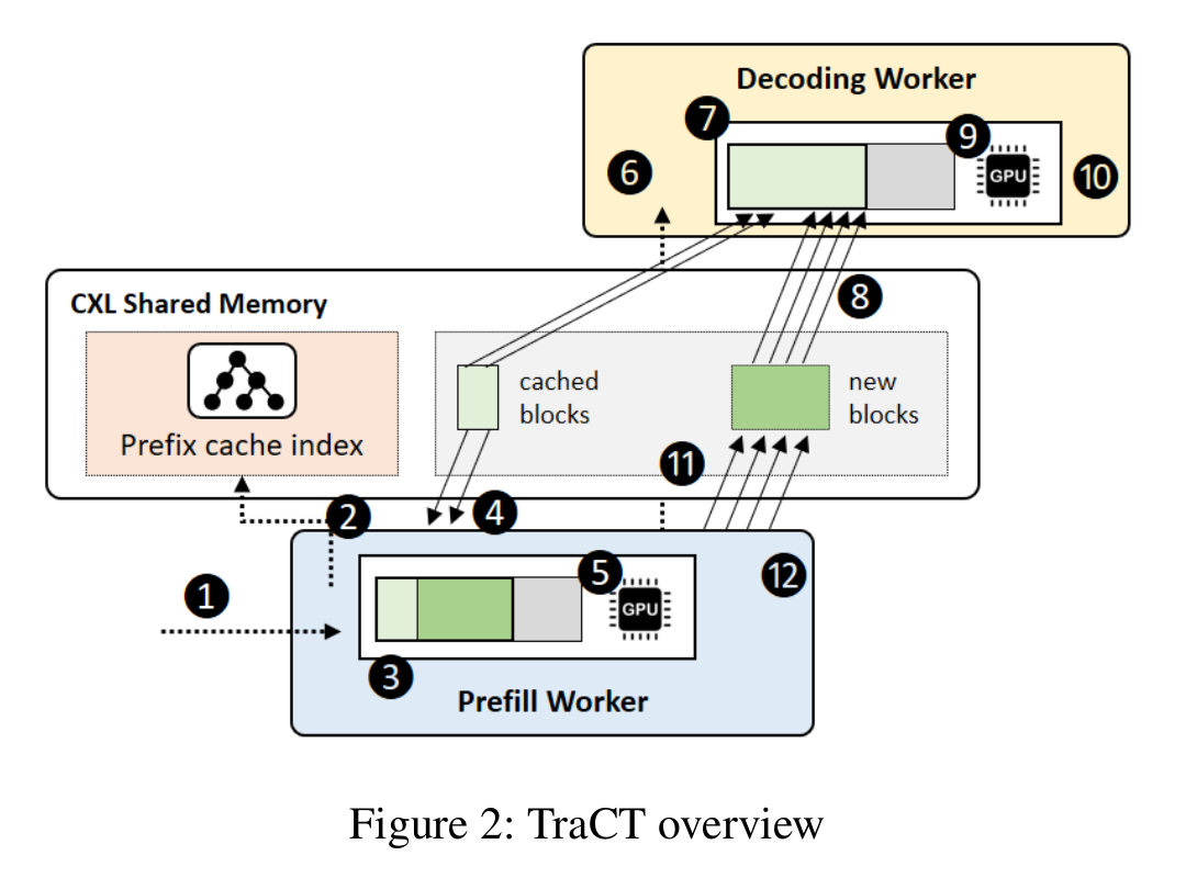
KV cache transfer and prefix caching with CXL shared memory. Source: TraCT, Figure 2
Use Case 2 — Memory Pooling and VM Consolidation
The second use case is memory pooling, which can directly improve datacenter economics.
The Stranded Memory Problem
Cloud servers bind a fixed number of CPU cores to a fixed amount of DRAM. Once customers rent all available CPU cores, the provider cannot sell the remaining DRAM separately. Conversely, when memory is exhausted first, the remaining CPU cores sit idle.
This is stranded memory: one resource is exhausted while another remains unused. The problem is especially visible in cloud environments that place multiple Virtual Machines (VMs) on each server.
How CXL Pooling Addresses It
CXL 2.0 pooling, introduced in Part 4, targets exactly this problem. It divides a large memory device into Multi-Logical Devices (MLDs), and a Fabric Manager (FM) dynamically assigns chunks according to each node’s demand.
The key is dynamic allocation rather than simultaneous sharing. At any moment, a chunk belongs to only one host, avoiding coherence conflicts and keeping the implementation relatively simple.
With this structure, every node no longer needs enough DRAM for its individual peak demand. Nodes can operate with less local DRAM and borrow only the missing capacity from the pool. The design benefits from the fact that all nodes are unlikely to reach their peak at the same time.
The VM scheduler can also place CPU and memory resources more independently.
Microsoft Azure’s Pond combined 75 days of VM placement traces from 100 Azure production clusters with performance measurements from 158 workloads running under emulated CXL latency. In an end-to-end simulation with memory latency at 2.22 times that of local DRAM, a 16-socket pool, and a 5% performance degradation target, Pond reduced total required DRAM capacity by 7%. The paper translates this into a 3.5% reduction in total cloud server cost.
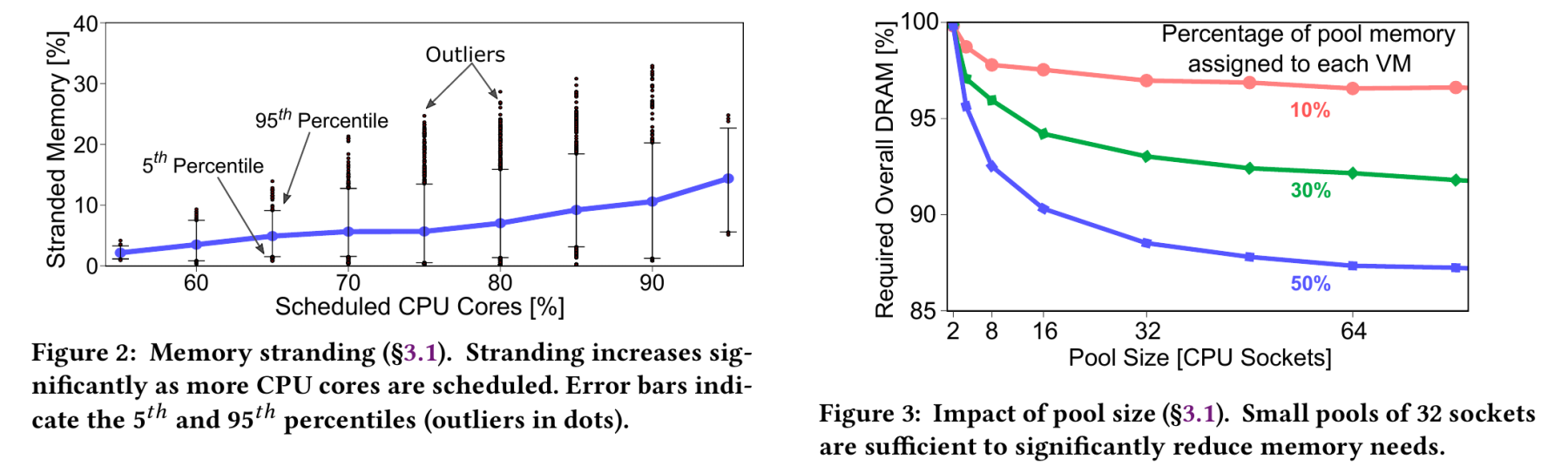
Azure stranded memory and DRAM savings by pool size. Source: Pond, Figures 2 and 3
Use Case 3 — Hot / Warm / Cold Tiering
The third use case is an operating model that connects the first two. Instead of treating CXL memory as a replacement for main memory, it places CXL one tier below it.
Why Tiering?
CXL memory is 2-3 times slower than DDR, so placing all data in CXL memory would be counterproductive. Instead, data is separated into tiers according to access frequency.
- Hot: frequently accessed data → nearby DDR
- Warm / cold: infrequently accessed data or data that mainly consumes capacity → more distant CXL memory
From the CPU’s perspective, CXL memory appears much like a “slower Non-Uniform Memory Access (NUMA) node.” The OS and runtime therefore manage which pages belong in each tier.
Automatic Tiering vs. Explicit Placement
Who manages tiering depends on the range of workloads the server supports.
- For general-purpose workloads, automatic OS tiering is convenient. Linux tracks page accesses, promotes hot pages to DDR, and demotes cold pages to CXL memory.
- For workloads with deterministic access patterns, such as LLM inference, the application can place data explicitly. The component that understands the data can decide, for example, that “active KV blocks stay in HBM, while reusable prefixes go to CXL.”
There is no universal definition of “access tracking” for automatic tiering. Implementations combine recency, access frequency, and idle time in different ways. For example, with its default settings, Linux DAMON_LRU_SORT classifies a memory region as hot when it is accessed during at least 50% of the observation interval, and as cold when it has not been accessed for 120 seconds. It then raises the LRU priority of hot pages and lowers that of cold pages so that cold pages are reclaimed first under memory pressure.
TPP turns that classification into movement between tiers. It asynchronously demotes cold reclaim candidates from local DDR to the CXL NUMA node. When a page in CXL memory is accessed, TPP first moves it to the active LRU list and promotes it to local DDR only if it remains hot at the next NUMA hinting fault. Requiring repeated evidence of hotness reduces page ping-pong caused by one-off accesses.
Vistara — CXL Tiering Validated in Production
Meta’s Vistara is a representative example of automatic tiering. Vistara connects DDR4 recovered from retired servers through a CXL Type 3 device. One AMD Turin server combines 768 GB of local DDR5 with 256 GB of CXL-attached DDR4 for a total of 1 TB.
Linux exposes CXL memory as a CPU-less NUMA node. Transparent Page Placement (TPP) and Transparent Memory Offloading (TMO) keep hot pages in local DDR5 and move cold pages to CXL-attached DDR4. This is memory expansion plus tiering within a single host.
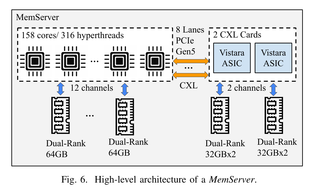
Vistara MemServer combining local DDR5 with CXL-attached DDR4. Source: Vistara, Figure 6
Meta showed that CXL can produce practical improvements at the server level. Enabling CXL increased the number of jobs or VMs per server by 33% in CI and development environments. For an ML workload, it reduced the number of required servers by 25% while increasing throughput by 4%.
Which Workloads Suit CXL?
The three use cases reveal a common set of conditions. CXL is well suited to workloads with the following characteristics.
- Capacity is the bottleneck, rather than latency.
- The workload contains data that can tolerate higher latency, such as cold data or a large working set.
- The access pattern is predictable enough for explicit placement.
By contrast, hot data on the critical path of every access, such as active KV blocks and weights used by attention at every step, still belongs in HBM or DDR. CXL does not replace those tiers. It expands the tier below them.
This is where HBF and CXL converge. HBF increases capacity between HBM and SSD next to the GPU. CXL expands capacity below local DRAM beside the CPU and across the system. Their physical positions and latencies differ, but both follow the same philosophy: place a slower but larger tier below fast, expensive memory.
Conclusion
Part 5 can be summarized in three points.
- Three use cases: KV cache offload / VM consolidation through memory pooling / hot-warm-cold tiering
- Common conditions: capacity-bound, tolerant of additional latency, and predictable access patterns
- CXL’s role: expanding the tier below expensive memory rather than replacing it
This series began by asking why SRAM, DRAM, HBM, and NAND cannot be collapsed into a single type of memory. The answer remained the same throughout: no single memory technology can maximize speed and capacity while minimizing cost.
HBF and CXL do not eliminate that trade-off. Instead, they keep immediately needed data in fast, expensive memory and place data needed later in slower, larger memory. HBF expands the tier near the GPU, while CXL expands the tier beside the CPU and at the system level.
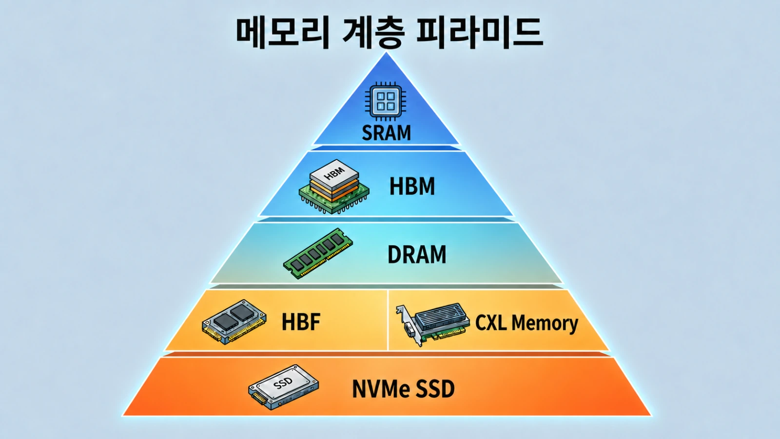
HBF and CXL Memory expand capacity in the memory hierarchy · AI generated image
Ultimately, no single memory can solve every problem. We must choose memory according to the characteristics of the data and combine tiers to meet each workload’s performance and capacity requirements.
That is because engineering has no single correct answer. It is a process of finding the best trade-off within the technology and budget available at the time, then adjusting it whenever new workloads and technologies emerge.
Across five parts, we examined why different kinds of memory exist and which problems new technologies are designed to solve. This concludes the Memory in the AI Era series. I hope it helped you better understand memory technology. Thank you for reading.
P.S.
As the memory hierarchy becomes more diverse, accelerator companies face increasingly complex and interesting problems. Building an optimized accelerator requires memory and compute logic, software, and algorithms to work together rather than remain isolated in separate domains.
HyperAccel works across hardware, software, and AI, bringing together talented people in every area. If you want to deepen a broad range of knowledge and grow with us, we would be glad to hear from you.
Careers: https://hyperaccel.career.greetinghr.com/en/guide
References
- Compute Express Link Consortium — Specifications
- Linux Kernel — CXL Driver Documentation
- D. Yoon et al., “TraCT: Disaggregated LLM Serving with CXL Shared Memory KV Cache at Rack-Scale,” 2025. arXiv:2512.18194
- H. Li et al., “Pond: CXL-Based Memory Pooling Systems for Cloud Platforms,” ASPLOS, 2023. DOI: 10.1145/3575693.3578835
- Linux Kernel, “DAMON-based LRU-lists Sorting”
- H. Al Maruf et al., “TPP: Transparent Page Placement for CXL-Enabled Tiered-Memory,” ISCA, 2023. arXiv:2206.02878
- N. Gholkar et al., “Vistara: Making CXL Real—Full Path from ASIC Design and OS Support to Hyperscale Deployment,” ISCA, 2026. Paper