Monads and Category Theory ① When Functions Do Not Compose

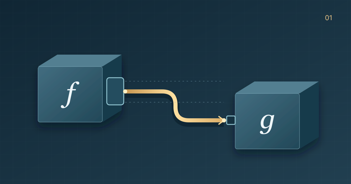
Hello, I am Jaeho Choi from the Compiler team at HyperAccel.

A monad has a reputation in functional programming as a concept that is unusually difficult to explain. Even if you have heard the name, it can be hard to say what it is and why we use it.

My reason for introducing monads is the beauty of function composition. We connect small functions to build a larger function, then connect that function to others. Being able to assemble a larger computation while understanding what each function does is one of the appeals of functional programming.

When we can pass one function’s result to the next, the task is straightforward. In real code, though, those connections do not always work as we intend. A function may produce no value or several results. We may also need to pass an updated state to the next step, or connect operations that interact with the outside world, such as reading a file. Can we preserve the ability to compose functions in sequence for these computations too?

This series begins where those connections break down. We will first write code that makes them work, then use the language of category theory to explore the laws that code satisfies and the mathematical structure within it. Along the way, we will work toward understanding what a monad is and how it lets us continue composing functions even when computations may produce no value or multiple results.

There is a reason for taking this approach. If you have looked for material on monads, you have probably encountered one of two barriers.

On one side stands the forbidding mathematical declaration, “A monad is just a monoid in the category of endofunctors.” Quoted without its original context, this unfamiliar mathematical vocabulary can exhaust readers before they even begin. On the other side are countless everyday analogies: “A monad is a burrito,” or “A monad is a box.” However many analogies you read, it can still be hard to find a clear answer to the basic questions: “Why should I learn about monads? Why does my code need this?”

Between mathematical declarations and everyday analogies lies code we can actually run. As we carry out computations and see exactly where their connections fail, the things those unfamiliar mathematical terms describe can begin to take a more concrete shape. By following the code, we will work toward reading a once-distant mathematical definition as a description of the connections we have built ourselves.

We will write that code in Lean 4. Lean 4 is both a functional programming language and an interactive theorem prover (ITP), which checks proofs of mathematical propositions. At first, we will use it to write and run functions. Later, we will use the same language to prove laws about the composition rules we have built. I will introduce the syntax as we need it in the examples.

In this article, we will connect two functions that may produce no value and build a reusable composition rule that works even when the functions change. Let us begin by connecting two ordinary functions.

1. Function composition: when outputs and inputs match

One way to manage complexity as software grows is to connect small functions.

Suppose we have one function that doubles a number and another that converts a number to a string. Applying them in sequence gives us a function that takes a number and returns a string representing twice that number. Whenever the output of the first function can serve as the input to the second, we can combine the two into a new function that performs a larger operation. In mathematics, this is called function composition, written $g \circ f$.

f : A → B
g : B → C
g ∘ f : A → C

In terms of types, we can combine two functions when the return type of the first matches the input type of the next. The function $g \circ f$ first applies $f$ to an input $a$, then applies $g$ to the result.

What is interesting here is that as long as the return type of $f$ matches the input type of $g$, we can connect the computations regardless of how either function is implemented. In our example, we could replace $f$ with a function that squares a number or adds one to it. Any function that returns a number can compose with our number-to-string function $g$. If we also have a function $h$ that encodes a string as UTF-8 bytes, we can continue composing: $h \circ g \circ f$.

When we write real programs, however, we find that this assembly does not always go so smoothly.

2. Missing output: when composition’s types no longer match

The usual mathematical function $f : A \to B$ returns some $b \in B$ for every input $a \in A$. Think of $\sin x$, $e^x$, or $x^2$. Such a function is called a total function.

In programs, however, we frequently encounter situations in which there is no output value: no corresponding $b$ is available for a given $a$.

Imagine writing a function that parses a user-provided string as a number. For the input "42", it can return the number $42$, but for "hello", it cannot return a valid number. Similarly, a lookup for a user account has no account information to return when the supplied ID is unregistered. A function whose output is undefined for some inputs is called a partial function.

Can we express a computation that cannot obtain a B for some inputs—a partial function—as a function defined for every input—a total function? Let us change one assumption: what if the absence of a value were itself represented by a value?

To do this, we change the return type from B to Option B. A value of Option B is either some b, containing a b : B, or none, representing the absence of a value. Even when there is no B to return, we can return none to express that fact. Python’s B | None, C++’s std::optional<B>, and Haskell’s Maybe B serve similar purposes. (Try looking up how your favorite language represents absence, too!)

We now define the function to return some b if it obtains a value for input a, and none otherwise. Every input has a corresponding Option B value, so this function has type A → Option B and is total. Option alone, however, does not tell us why the value is absent.

Let us connect two stages of such a computation. First, we parse an input string as a natural number; then we take that number’s reciprocal. With "42", we can complete both stages. With "hello", the first stage cannot obtain a number. With "0", parsing succeeds, but the second stage cannot obtain a reciprocal.

Call the first function $f$ and the next one $g$. Since either may fail to obtain a value, their types are:

f : A → Option B
g : B → Option C

The problem appears when we try to compose them as before.

g (f a)  -- Compile error: Option B cannot be used where B is required

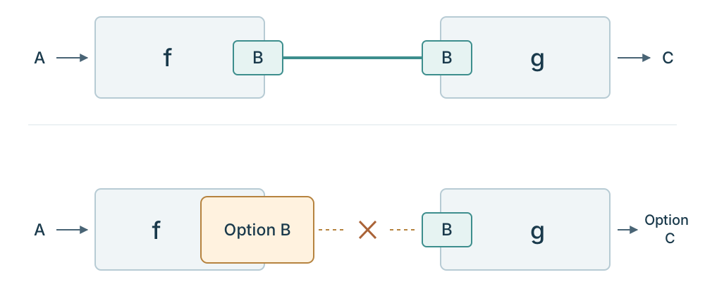
$f$ hands us an Option B—a box (or a burrito) accounting for possible absence—while $g$ requires a $B$ value.

We therefore cannot directly define ordinary composition $g \circ f$ for $f : A \to \text{Option } B$ and $g : B \to \text{Option } C$.

How can we compose functions that may produce no value? How do programmers usually handle this mismatch?

3. Connecting two computations with branching

We cannot use $g \circ f$ directly, but the behavior we want from the connection is clear. If $f\,a$ is none, the overall result should be none. If it is some b, we should pass that $b$ to $g$ and use $g\,b$ as the result. For now, let us write this new composition as $g \star f : A \to \text{Option } C$.

Here is how we can write it using Lean’s pattern matching. We will add one more stage, $h : C \to \text{Option } D$.

def runOption {A B C D : Type}
    (f : A → Option B) (g : B → Option C) (h : C → Option D)
    (a : A) : Option D :=
  match f a with
  | none => none
  | some b =>
    match g b with
    | none => none
    | some c => h c

This code computes exactly the result we want. If $f\,a$ is none, it stops at the first branch; if it is some b, it runs $g\,b$. If $g\,b$ is also none, it stops, and only if it is some c does it continue to $h\,c$. This is enough to write a single pipeline.

But what the branches do is independent of the particular computations performed by $f$, $g$, and $h$. We have written a connecting rule directly inside runOption: stop if the previous result is absent; otherwise, pass it to the next function. We need the same rule when connecting other functions or adding more stages.

Our goal goes beyond shortening this particular runOption: we want a method of composition that takes $f$ and $g$ and produces another function of type $A \to \text{Option } C$. This requires extracting the repeated branching at call sites into an operation between two functions. Let us first see whether an existing operation can do the job.

4. Nested contexts: why map alone is not enough

Developers familiar with functional programming might ask:

“Doesn’t map apply a function to the value inside a container? Couldn’t we use (f a).map g?”

Here, $α$ and $β$ each stand for an arbitrary type. Option.map takes a function of type $α \to β$ and applies it to the value inside an Option α. Its type and behavior in the two cases are:

Option.map : (α → β) → Option α → Option β

Option.map g none     = none
Option.map g (some b) = some (g b)

Since $g : B \to \text{Option } C$, applying it inside some b gives some (g b). This wraps Option C in another layer, producing Option (Option C). Applying it to the result of f a gives:

f a               : Option B
g                 : B → Option C
(f a).map g       : Option (Option C)

For example, if $f\,a = \text{some }0$ and $g\,0 = \text{none}$, then (f a).map g is some none, rather than none. A value is present, but that value is itself “absent.” The two layers retain the fact that the first computation produced a value while the second did not.

We wanted a single Option C result: a value is either present or absent. What we have instead is Option (Option C), one wrapper inside another.

It is like opening a box to find another box inside, as with Russian nesting dolls. map takes the inner $B$ and passes it to $g$, but does not remove the new wrapper ($\text{Option } C$) that $g$ itself produces.

Nor can we directly apply the next operation, $h : C \to \text{Option } D$, to this result. The value inside the outer Option is an Option C, whereas $h$ needs a $C$.

5. Building a composition rule with join and bind

We have just obtained an Option (Option C). To return to the Option C we wanted, we need to remove the outer Option layer. If the outer value is none, return none; if it is some result, return the inner result unchanged. This operation has type Option (Option C) → Option C and is called Option.join in Lean. Because it reduces a nested context to one layer, its behavior is often described as flattening. We will use its operation name, join.

Let us apply join to the map result from Section 4. If $f\,a$ is none, $g$ is not run and the result is none. If $f\,a$ is some b, map produces some (g b), and join removes the outer some to return $g\,b$.

((f a).map g).join : Option C

if f a = none,    the result is none
if f a = some b,  the result is g b

The two branches we wrote explicitly in Section 3 have reappeared in this expression. In particular, when $g\,b$ is none, map produces some none, but join turns it into none. If we open the outer doll and find that the inner one is empty, the final result is simply “empty.”

Combining map, which applies a function to an inner value, with join, which removes one layer of nesting, gives an operation commonly called flatMap or bind. You will encounter it as Option.bind in Lean, flatMap in Java and Swift, and and_then in Rust and C++. In our code, we will use Lean’s name, bind.

We can express the relationship between the operations as follows.

m.bind g = (m.map g).join

If m is none, both sides produce none. If it is some b, bind returns g b directly. On the right, map produces some (g b), which join reduces to g b. Thus the two computations produce the same result for any Option value m and next function g.

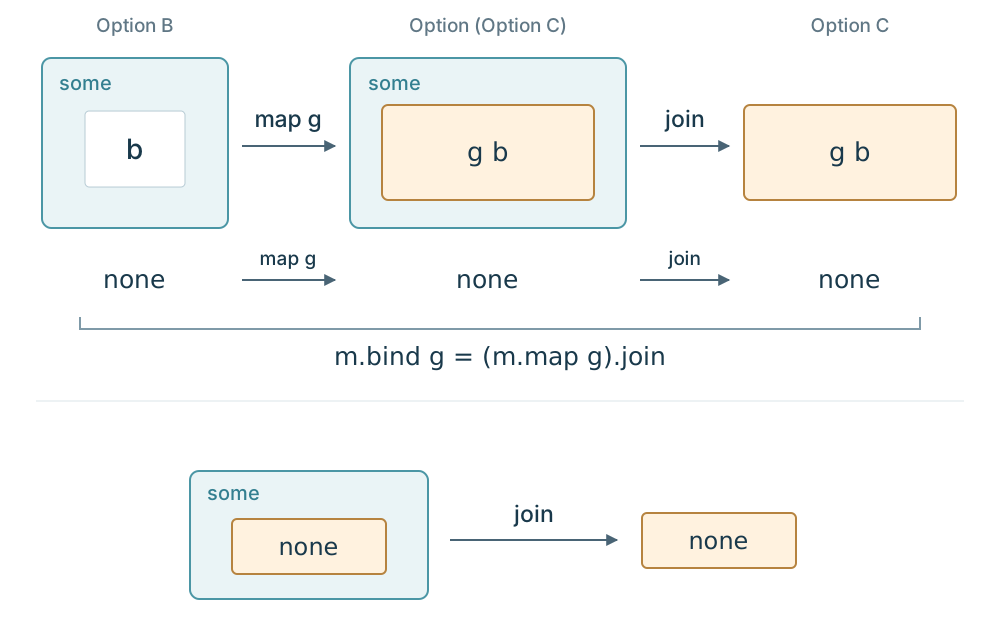
Here, m : Option B and g : B → Option C. bind provides both steps together, while join removes one layer from an already nested Option. Later, in the formal definition of a monad, we will encounter this relationship again in the general form bind m g = join (map g m).

Option.bind : Option B → (B → Option C) → Option C

composeOption (f : A → Option B) (g : B → Option C) : A → Option C
composeOption f g a = Option.bind (f a) g

Option.bind connects an existing Option B value to the next function. Using it, we define composeOption, an operation that takes two functions and produces a new function. For each input $a$, it runs $f$, then connects the result to $g$ using bind. The composition we previously wrote as $g \star f$ is exactly composeOption f g.

Notice that the result of composition is itself a function of type A → Option C. If another function h : C → Option D follows, we can connect this result to h using the same operation.

composeOption f g                  : A → Option C
composeOption (composeOption f g) h : A → Option D

Where we previously wrote another branch for each additional function, we can now reuse the composition operation we have already built. Each function handles its own computation; composeOption handles stopping when a value is absent and passing it to the next function when it is present.

6. Checking composition in Lean 4

We will now define the three ways of connecting functions in Lean 4 and compare their results on representative inputs.

We will define parseNat, which parses a string as a natural number, and reciprocal, which represents the reciprocal of a nonzero natural number as a string of the form "1/n". The example focuses on absence and function connections, rather than numerical operations on fractions.

-- Monads and Category Theory ① When Functions Do Not Compose
-- Lean 4.32.1. Runs without additional libraries.

-- 1. Two functions that may produce no value
def parseNat (s : String) : Option Nat :=
  s.toNat?

def reciprocal (n : Nat) : Option String :=
  if n == 0 then
    none -- No reciprocal is represented for zero
  else
    some s!"1/{n}"

We define the connecting rule as composeOption. For comparison, we will also write out the branching from Section 3 and the map followed by join from Section 5.

-- Call the next function according to the previous result
def composeOptionByMatch {A B C : Type}
    (f : A → Option B) (g : B → Option C) : A → Option C :=
  fun x =>
    match f x with
    | none   => none
    | some b => g b

-- Express the same rule using Option.bind
def composeOption {A B C : Type}
    (f : A → Option B) (g : B → Option C) : A → Option C :=
  fun x => (f x).bind g

-- The same rule: apply map, then flatten one layer with join
def composeOptionByJoin {A B C : Type}
    (f : A → Option B) (g : B → Option C) : A → Option C :=
  fun x => ((f x).map g).join

Now let us compose the two functions.

def parseAndReciprocal : String → Option String :=
  composeOption parseNat reciprocal

parseAndReciprocal specifies only which two functions to connect. composeOption handles stopping when the previous result is absent and passing it to the next function when it is present. We can use the same rule unchanged to connect other functions.

#eval is a Lean command that executes the expression after it and displays the result. We can use it to inspect an input that succeeds, along with inputs for which a value is absent at either stage.

#eval parseAndReciprocal "42"  -- some "1/42"
#eval parseAndReciprocal "0"   -- none       (No reciprocal is represented for zero)
#eval parseAndReciprocal "foo" -- none       (Parsing failed)
#eval (parseNat "0").map reciprocal -- some none (Two layers before join)

Having inspected the results with #eval, we will now use #guard to check whether they satisfy the conditions we expect. #guard passes without an error when the condition after it is true, and makes Lean report an error when it is false. Here, == compares two computed results for equality.

The first line below checks whether composeOptionByMatch, implemented with branching, and parseAndReciprocal, implemented using bind, produce the same result for the input "42". The remaining lines similarly compare against another implementation or an expected result. These are some of the checks; the Playground contains the full set for all three inputs.

#guard composeOptionByMatch parseNat reciprocal "42" == parseAndReciprocal "42"
#guard composeOptionByJoin parseNat reciprocal "0" == parseAndReciprocal "0"
#guard parseAndReciprocal "foo" == none

To modify the code and run it yourself, open this example in the Lean 4 Playground.

composeOptionByMatch explicitly handles none and some b, while composeOptionByJoin applies map followed by join. Option.bind expresses the same connection in one line. The #guard checks comparing these implementations on representative inputs verify examples; they do not prove equality for every input.

• With "42": parsing succeeds ($\text{some } 42$) $\to$ a fraction representation is produced ($\text{some } “1/42”$).
• With "0": parsing succeeds ($\text{some } 0$) $\to$ the second function returns none.
• With "foo": parsing fails ($\text{none}$) $\to$ the second function is never run, and $\text{none}$ is returned immediately.

We handled absence inside the composition rule, composeOption, without manually checking it at every call. join flattens both an outer none and a some none whose inner value is absent to none. Consequently, the final result alone cannot tell us which stage failed to produce a value.

An aside: proving an equation in Lean

So far, we have run specific inputs and checked their results. With Lean, we can go a step further and prove that two computations agree for any input and function. Let us prove m.bind g = (m.map g).join, the equation we checked by considering both cases in Section 5.

This uses the interactive theorem prover capability introduced earlier. In Lean, we can write both a claim and the reasoning that establishes it. As we write the steps of a proof, Lean checks that each step is valid and tells us what remains to be proved. In the code below, example declares the claim to prove, and the commands after by construct its proof.

example {B C : Type} (m : Option B) (g : B → Option C) :
    m.bind g = (m.map g).join := by
  cases m <;> rfl

cases m splits the proof into the cases where m is none and where it is some b. <;> applies the following rfl to both cases. rfl checks that both sides of the equation reduce to the same expression according to their definitions. Since both cases are proved without choosing a specific b or g, Lean can verify that the equation holds for arbitrary m and g.

7. The next question: laws of the composition rule

At first, we could not pass the Option B returned by the first function directly to the next. We can now express a rule in composeOption: stop when a value is absent, or pass it to the next computation when it is present. The rule remains reusable even when the functions change. The monads we will study bring together operations that connect computations in this way and the laws those operations must obey.

Will this rule give consistent results across multiple stages? We need to check whether either grouping of three functions gives the same result, and whether a function that simply wraps its input in some leaves composition unchanged.

In the next article, we will build a composition for List, where a single input can produce multiple results. Comparing these two kinds of computation—absence and multiple results—will help us see what their compositions have in common. We will then ask whether matching the types of a composition is enough, and prove in Lean 4 that our Option composition satisfies associativity and the identity laws.