
Introduction
Hi, I’m Sinhyun Park from the LLMOps team at HyperAccel.
The Ceph Deep-Dive series takes apart the internals of Ceph, an open-source distributed storage system, one piece at a time. It is written for engineers who are meeting Ceph for the first time.
This first part covers Controlled Replication Under Scalable Hashing(CRUSH), the data distribution algorithm that Ceph is built on. The explanation follows the paper CRUSH: Controlled, Scalable, Decentralized Placement of Replicated Data(SC'06).
Background
Object-based Storage
Object storage stores and manages data as independent objects, not as files or blocks.
- A conventional file system manages data through metadata such as the directory tree and inodes.
- An inode (index node) is a data structure that holds a file’s size, permissions, and the locations of its data blocks.
- Object storage manages data as an object ID (key) and an object (value).
bucket
├── logs/2026/09/09/a.json
├── logs/2026/09/09/b.json
└── model/llama/weights-001
- The storage structure is simple, scales out well, and keeps replication cheap.
- Large object-based distributed storage splits data into small objects and spreads them across many disks.
- Large reads and writes are served by many storage devices in parallel.
- Replicas and erasure coding shards are spread out to survive failures.
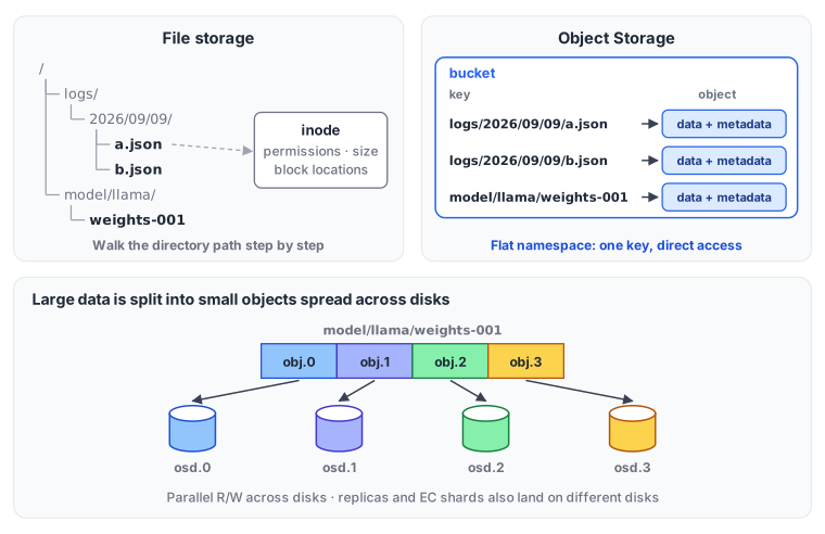
The core problem of object storage is which device should store each of a huge number of objects?
Challenge
Spreading objects across many devices raises three problems. Each subsection ends with the question that problem poses.
Q1. Object Metadata Scalability
In Ceph, the unit that actually stores data on a disk is called an Object Storage Daemon(OSD). The example below stores the object-to-OSD mapping in a table.
object-A → osd.1
object-B → osd.7
object-C → osd.3
...
- Storing the mapping for every object to every disk creates a metadata load that hurts scalability and availability.
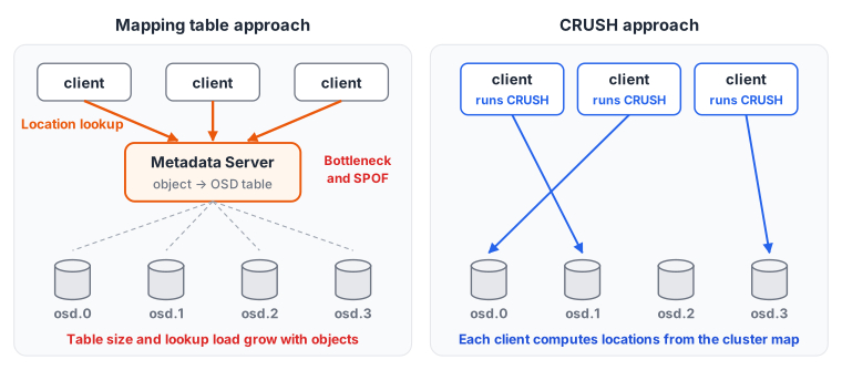
- On the left, every request goes through the metadata server, which becomes both a bottleneck and a single point of failure (SPOF).
- On the right is the CRUSH approach covered in this post. Each client computes the location itself, so no central lookup is needed.
This leads to the first question CRUSH has to answer.
Can any node compute an object’s location without storing placement information?
Q2. Reliable Replica Placement
Spreading data across devices does not by itself make it safe.
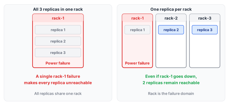
- As on the left, if all replicas land in the same rack domain, a power failure makes the data unreachable.
- As on the right, with one replica per rack, the remaining replicas keep the data reachable even if one rack goes down.
- Replica placement must take several failure domains into account, such as rack, power, site, and server.
The second question is how to reflect failure domains in placement.
Can the placement process distinguish and structure failure domains?
Q3. Dynamic Cluster & Data Rebalancing
# N = number of devices
device = hash(object_id) % N
- Hash-based placement uses randomness to spread objects evenly across devices.
A storage cluster changes constantly as devices are added, removed, or replaced. When a device fails, its data has to move to other devices.
hash(x) % 10 -> hash(x) % 11 ...?
The example below shows how the locations of 12 objects change when the cluster grows from 4 devices to 5.
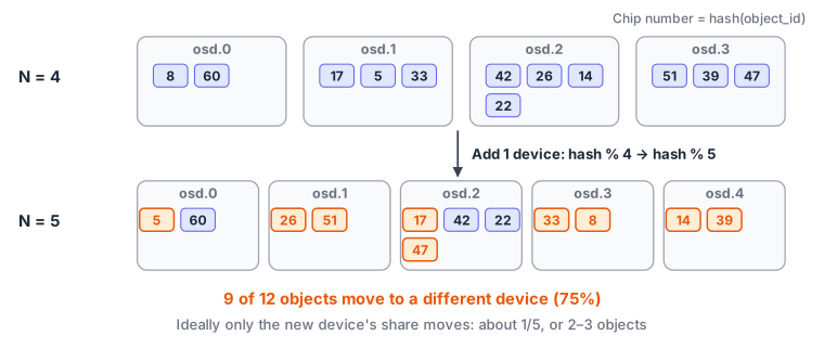
- When the number of devices changes, most existing object mappings change. The result is massive relocation.
The last question is about how much data moves when the cluster changes.
Can data be redistributed as the cluster changes while keeping data movement to a minimum?
Solution: CRUSH Overview
CRUSH computes object placement from a hash function instead of storing it in a mapping table.
object_id -> CRUSH(object_id, cluster_map, placement rule) -> [device1, device2]
- Because CRUSH computes placement with a hash function, data is distributed pseudo-randomly.
- Yet it is a deterministic algorithm: the same
(object_id, cluster_map, placement rule)input always produces the same output.
Deterministic Pseudo-random Placement
CRUSH(X) = always OSD 7
- For object
X, CRUSH always returns OSD 7.
X, Y, Z -> CRUSH(X), CRUSH(Y), CRUSH(Z) -> OSD 7, 3, 5
- Across many objects, CRUSH results are spread randomly over many devices.
Without a central placement server, every node can compute an object’s location on its own.
Cluster Map
CRUSH represents the physical layout of a cluster as a weighted hierarchy tree.
root
└── row
    └── cabinet
        └── shelf
            └── device (leaf disk)
- Tree leaves are the devices that actually store data.
- Tree nodes organize devices into a hierarchy and are called
buckets.- The paper’s example uses a four-level bucket hierarchy: root > row > cabinet > shelf.
- Devices and buckets each have their own weight.
- Device weight: the relative amount of data the device should store. It is usually proportional to capacity.
- Bucket weight:
Σ child weights, the sum of the weights of its child buckets and devices.
If the device weights in a bucket are as follows, the devices store data in a 1 : 2 ratio.
osd.1 weight = 1
osd.2 weight = 2
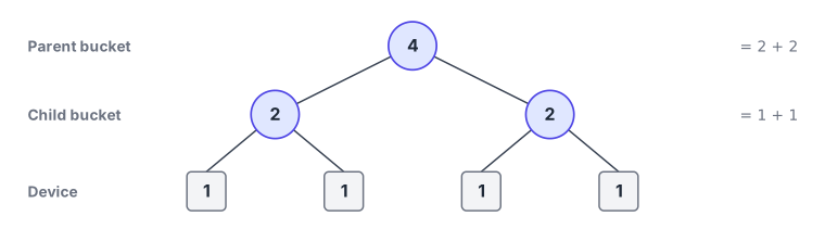
- The parent bucket’s weight is the sum of its child bucket weights
(2+2). - Each child bucket’s weight is the sum of its device weights
(1+1).
By mapping real failure domains to hierarchical buckets in the cluster map, such as IDC sites, racks, and network switches, you can model the physical environment.
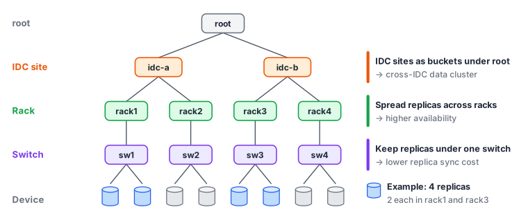
- Assign different IDC sites to buckets under root to build a cross-IDC data cluster.
- Assign each rack to an upper-level bucket and spread replicas across different racks. If one rack goes down, replicas in the other racks survive, which raises availability.
- Assign each switch to a lower-level bucket and keep the replicas within a rack under the same switch. Replicas can then sync without crossing switches, which cuts synchronization cost.
- For example, with four replicas, place two each in rack1 and rack3, as the blue devices show, and keep the two in each rack under the same switch.
Placement Rule
A placement rule decides how to traverse the cluster map and where to place replicas.
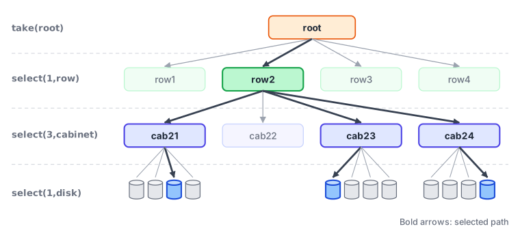
For example, suppose the cluster map has three bucket levels: row, cabinet, and disk.
root
 ↓
row1    row2
 ↓       ↓
cab21   cab23   cab24
 ↓       ↓       ↓
disk    disk    disk
- You can keep replicas in the same row to reduce rebalancing cost.
- Or you can spread replicas across different rows to raise availability.
CRUSH expresses these replica placement policies with its TAKE / SELECT / EMIT functions.
take(root)
select(1,disk)
emit
take(root)
select(1,row)
select(3,cabinet)
select(1,disk)
emit
A placement rule can separate replicas across one failure domain while confining them within another.
Placement Algorithm
TAKE / SELECT / EMIT
The placement algorithm recursively descends the cluster map according to a placement rule made of TAKE / SELECT / EMIT, and finds suitable disks for an object ID.
TAKE(a)
SELECT(n, t)
EMIT

- i = current working vector
- b = bucket currently being descended
- o = candidate selected from b
root
 ↓
row1    row2
 ↓       ↓
cab21   cab23   cab24
 ↓       ↓       ↓
disk    disk    disk
TAKE(a) puts the entry point where the traversal starts into the working vector i.
take(root) -> [root]
SELECT(n,t) selects n items of type t under each item in the current working vector i and adds them to i. The pseudocode below illustrates how it works.
[root] -> select(2,row)

for r=1 in range(N):
- r=1. i: root, b: root, o: row1 (type(o) = row, found) -> [row1]
- r=2. i: root, b: root, o: row2 (type(o) = row, found) -> [row1, row2]
- SELECT descends recursively until it reaches the target type.
select(1,disk) - i: [row1, row2]
- r=1. i: row1, b: row1,  o: cab21 (type(o) != disk, descend)
- r=1. i: row1, b: cab21, o: disk2107 (type(o) = disk, found) -> [disk2107]
- Within a bucket, the candidate is chosen by a hash-based selection function
c(r,x)that takes the indexrand the object IDx.c(r,x)depends on the bucket algorithm, which is covered in the Bucket Algorithm section.
b.c(r,x) -> cab21.c(1,21H3T#) -> disk2107
EMIT appends the current working vector i to the final placement result.
emit -> [disk2107, disk2313]
The whole process, seen from the working vector i, looks like this.
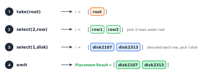
Failure Handling
In collision, crushed, and overload situations, a candidate chosen by CRUSH may not be fit to store data, so CRUSH has to search again.
- Collision: the candidate for index
rhas already been selected. Duplicate placement must be avoided. - Crushed: the selected candidate is unusable, for example because the disk has failed.
- Overload: the selected candidate is overloaded and load needs to be balanced.
In all three cases, CRUSH searches again and picks a different candidate.
To pick a different candidate, the retry passes a mutated index
r'toc(r,x)instead ofr.
- CRUSH counts
f, the total number of failures in the SELECT, andfr, the number of failures for a specific replica.
select(1,disk) - i: [row1, row2], f:0,
- [r=1, f:0]. i: row1, b: row1,  o: cab21
- [r=1, f:0]. i: row1, b: cab21, o: disk2107 (disk2107 Fail!!)
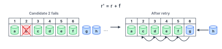
- When the selected candidate fails, CRUSH increments the failure count (
f += 1) and mutates the index tor' = r + f.- As the figure shows, when slot 2 fails, the replicas after it shift left by one and the next candidate, g, fills slot 6.
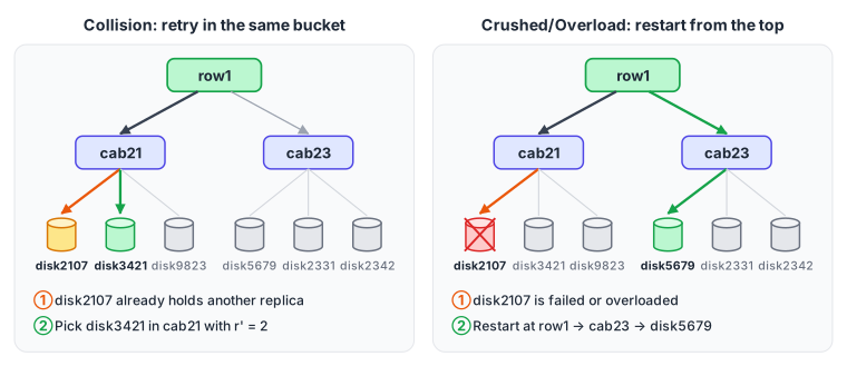
- On a collision, it searches again inside the bucket currently being descended.
select(1,disk) - i: [row1, row2], f:0,
- [r=1,  f:0]. i: row1, b: row1,  o: cab21
- [r=1,  f:0]. i: row1, b: cab21, o: disk2107 (disk2107 Collision!!)
- [r'=2, f:1]. i: row1, b: cab21, o: disk3421
- On crushed or overload, it goes back to the working vector item where the descent started and searches again.
select(1,disk) - i: [row1, row2], f:0,
- [r=1,  f:0]. i: row1, b: row1,  o: cab21
- [r=1,  f:0]. i: row1, b: cab21, o: disk2107 (disk2107 Overload!!)
- [r'=2, f:1]. i: row1, b: row1,  o: cab23
- [r'=2, f:1]. i: row1, b: cab23, o: disk5679
Collision handling vs Crushed/Overload handling
- Collision: the disk itself is fine, so CRUSH only needs to spread replicas within the bucket to avoid duplicates.
- Crushed/Overload: CRUSH steers data into a different bucket branch so it reaches a healthy disk.
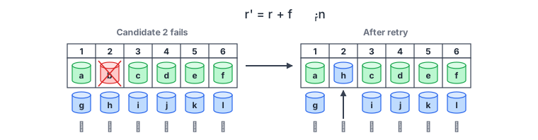
fr, the failure count for a specific replica, is used to keep positions stable when replica rank matters, as in erasure coding.- Like
f,fris incremented on every failure, but it is reset to 0 each time a candidate search finishes. - During mutation, CRUSH adds
fr x N,frmultiplied by the number of candidates, instead offritself. This preserves position information: as the figure above shows, only the failed slot 2 changes to h, and the other replicas stay in place.
- Like
select(1,disk) - i: [row1, row2], f:0,
- [r=1,  fr:0]. i: row1, b: row1,  o: cab21
- [r=1,  fr:0]. i: row1, b: cab21, o: disk2107 (disk2107 Collision!!)
- [r'=3, fr:1]. i: row1, b: cab21, o: disk9823
Cluster Change & Data Movement
When a device is added, removed, or reweighted, the cluster map changes and data is rebalanced.
Add / Remove / Reweight
B1(1) B2(1)
B1(1) B2(2)
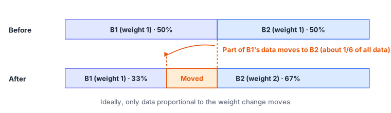
- When a disk’s weight changes as in the example above, data has to move to match the new ratio (
B1 → B2). - Ideally, only the data matching the weight change migrates from
B1toB2. - CRUSH does not delete or copy data itself. Instead, it guides data toward its desired placement under the updated cluster map.
Hierarchical Remapping
     root
    /    \
  A(1)   B(2)
         /  \
     B1(1)  B2(1)
     root
    /    \
  A(1)   B(3)
         /  \
     B1(1)  B2(2)
- In a hierarchy, however, not only the weight distribution of
B1andB2changes, but also that of the upper level,AandB.- So data moves in the
A → Bdirection at the same time asB1 → B2.
- So data moves in the
- Here, the placement decisions at root and at B are independent, which can cause unintended data movement.
- The ideal path for the moving data is
A → B → B2. - However, some of the data that moves from
AtoBmay land onB1. - Then
B1, whose share should shrink, actually gains data and drifts from the target weight distribution. - As a result, additional
B1 → B2movement occurs to restore the target weight distribution inside B.
- The ideal path for the moving data is
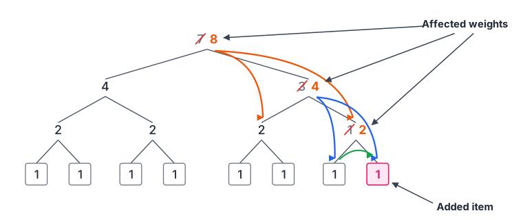
In other words, data does not move straight to the leaf whose weight increased. Different objects are remapped independently at each level of the hierarchy, which can cause extra, unintended data movement.
The cluster map should therefore be designed so that remapping caused by cluster map changes is minimized.
Bucket Algorithm
Each bucket in the cluster map has its own
c(r,x)implementation for choosing a candidate.
- Each bucket algorithm trades off placement computation cost against cluster change cost.
- Choosing an algorithm that fits the bucket keeps both costs low.
| Bucket | Mapping Cost | Addition | Removal |
|---|---|---|---|
| Uniform | O(1) | Poor | Poor |
| List | O(n) | Optimal | Poor |
| Tree | O(log n) | Good | Good |
| Straw | O(n) | Optimal | Optimal |
Uniform
Distributes data across items with perfectly equal probability.
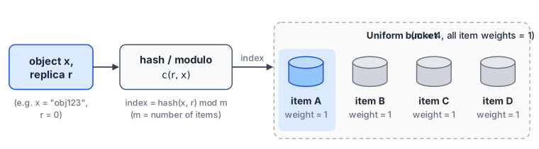
- It divides the hash value by the number of items and picks each child item with equal probability.
c(r,x) = hash(r,x) mod m, wheremis the number of items.
- It is used when all items have the same weight, and it computes placement the fastest (
O(1)). - In exchange, changing the number of items changes most object mappings, so its rebalancing cost is the worst.
List
Keeps the existing weight distribution as intact as possible by adding items to the front, like a stack.
- All items form a linked list, and items are considered one by one from the most recently added, each with a conditional probability. The pseudocode is below.
# hash values are normalized to [0, 1),
# remaining_weights holds the weights from the current item to the tail.
for item, weight in items:
    if hash(x, r, item) < weight / sum(remaining_weights):
        return item
- If the hash value is smaller than the current item’s share,
weight / sum(remaining_weights), that item is selected. Otherwise the search moves to the next item.
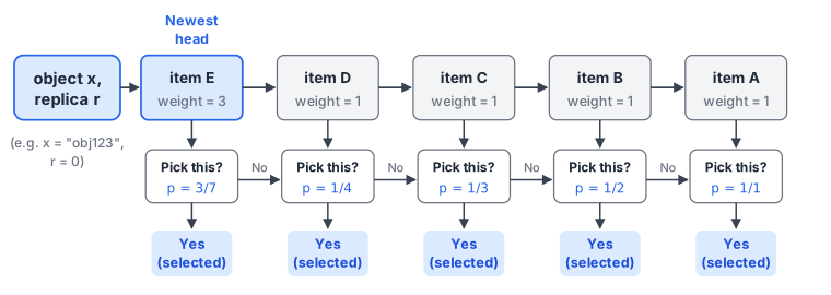
- Because it walks the items in order from the head, placement costs
O(n). - When a new item is added, every object except those that now pick the new item keeps its mapping.
Conditional probabilities, old list: E(3/7)  -> D(1/4) -> C(1/3) -> B(1/2) -> A(1/1)
Conditional probabilities, new list: F(4/11) -> E(3/7) -> D(1/4) -> C(1/3) -> B(1/2) -> A(1/1)
- After the added item
F, the conditional probabilities are the same as before. - In contrast, when an item in the middle or near the tail is removed, most conditional probabilities change, so object mappings change significantly.
Conditional probabilities, old list: E(3/7) -> D(1/4) -> C(1/3) -> B(1/2) -> A(1/1)
Conditional probabilities, new list: E(3/6) -> D(1/3) -> C(1/2) -> B(1/1)
Tree
Instead of walking a list in one direction, it narrows the search range recursively to pick an item.
- The probability-based selection is the same as in List, but the data structure is a weighted binary tree.
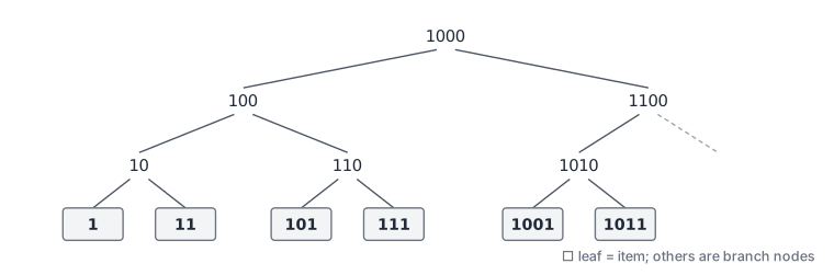
- All items live in the leaves, and internal nodes only branch.
- The leftmost leaf always has label 1. Leaf labels are odd, and branch node labels are even.
- Each time the tree grows by one level, the old root becomes the left child of a new root, and the new root’s label is the old root’s label shifted left by one bit (
100 → 1000). - As a result, existing node labels never change as the tree grows, so the paths to existing items stay the same.
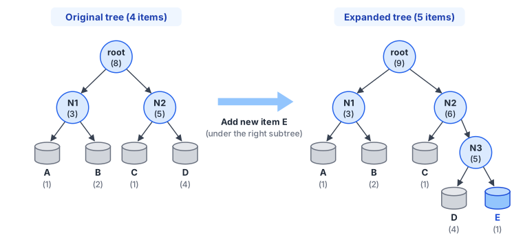
- Item lookup descends from the root, going left or right with probabilities based on the weight ratio.
- When adding an item expands the tree, a lot of data moves to the new branch, but most mappings in existing branches are preserved.
- Because it is a tree, placement costs
O(log n).
Straw
Unlike List and Tree, where only some items take part in a selection, every item is a candidate every time.
- It computes a score for every item with a hash function and picks the highest. The score corresponds to the length of the straw each item draws.
- In the paper, Straw is
c(r,x) = max_i( f(w_i) · hash(x, r, i) ).f(w_i)is a straw length factor that grows with weight. - Ceph now uses an improved version, straw2, by default. It computes the score as
ln(hash(x, r, i)) / w_i. - Because hash values lie in
(0, 1],lnis at most 0. A larger weight pulls the score closer to 0, which makes the item more likely to win.
- In the paper, Straw is
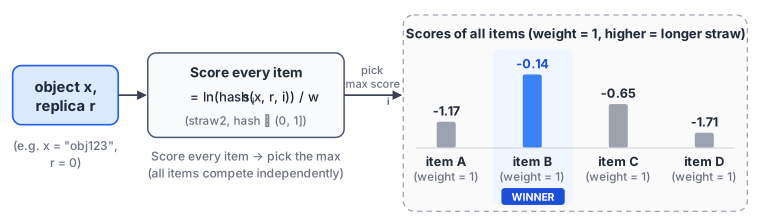
- Every item competes independently every time, so data moves only when the winning item changes after a cluster change.
- However, every selection must score every item, so placement costs
O(n).
Choosing a Bucket Algorithm
- Disks have identical capacity and performance, and the cluster rarely changes: use Uniform, which has the fastest placement.
- The cluster keeps growing and disks are never removed: use List, which makes adding items cheap, and consider Tree at large scale.
- Disks are added and removed often, and rebalancing cost must be minimal: use Straw, which moves less data at the cost of slower placement.
- The cluster changes and is quite large: use Tree, which balances placement cost and data movement cost.
Wrapping Up
This post looked at how CRUSH computes object locations without a mapping table. The cluster map structures failure domains, placement rules express replica placement policies, and bucket algorithms balance computation cost against data movement cost.
The next part covers the overall design of Ceph, which runs on top of CRUSH.
References
- Sage A. Weil, Scott A. Brandt, Ethan L. Miller, Carlos Maltzahn. CRUSH: Controlled, Scalable, Decentralized Placement of Replicated Data. SC'06.